9 Data Preparation – Business Analytics Course

9.1 Data Manipulation, Transformation and Cleaning

9.2 Reshaping Data

A significant challenge with analytics is that the required data is rarely collected with a view to perform analytics. It is mostly intended to support transaction processing, or managing operations. Data is often ‘dirty’, meaning data can be missing, duplicated, in the wrong formats, in different data sources/files, have character-set issues, require additional mappings, and so on.

Data analysts spend a great deal of time cleaning and preparing data for analysis. In traditional business intelligence contexts, data cleaning and transformations are referred to as ETL processes (Extract-Transfer-Load).

Data scientists often set up defined ‘data pipelines’ – a series of data processing steps that ingest and bring data to a desired format and shape.

During the rest of this chapter, we will see how we can select and filter data, understand data types, add and delete columns in tabular data, replace values, deal with missing values, and more. We will do all of this primarily using pandas, and also a few other libraries.

So what is it that we do when we reshape and clean data? While of course this would almost always depend upon the data and what shape we are trying to get it to, there are several common actions that we have to perform that we should know about.

Select columns: with a view to reducing the number of data fields we have to deal with by dropping the un-needed columns and retaining only the rest.
Selecting rows: filter out observations based on some criteria as to retain only the observations of relevance to us.
Change data types: Dates or numbers may be formatted as strings, or categories may appear as numbers. We may need to change the data types to suit our needs.
Add columns: We may need to insert new calculated columns, or bring in data from other data sources as additional features or columns to our dataset.
Reorder or sort columns and rows: We may need to rearrange the columns and rows in our data to support understanding and presentation.
Rename fields: to remove spaces, special characters, or renaming them as to be more humanly readable.
Remove duplicates: We may need to remove duplicate observations.
Replace values: Often we may have a need to change one value in the data for another, for example, replace United Kingdom with the letters UK.
Bin numerical data: We may need to convert numerical data to categories by grouping them into bins. For example, we may like to call homes with 4 to 6 bedromms as ‘Large’, converting a numerical column to a binned category.
Extract unique values: to understand the data better.
Combine: with other data sources as to enrich the information we already have.
Missing values: We might like to fill in missing values for a more complete dataset, or remove data with missing values from our dataset.
Summarize: using groupby or pivot functions to summarize or ‘elongate’ the data as to make it more suitable for use in subsequent analysis. (Also called melting and casting)

In the end, we want to have the capability to twist and shape data in the way we need it for our analysis. Python provides us tools and libraries that give us incredible flexibility in being able to do so.

Missing values deserve a special mention. We will also look at length on missing values, where we don’t have all the data for every observation. What are we to do in such a case? Should we ignore the observations that are missing any data, and risk losing the data that we have, or try to compensate for the missing data using some smart thinking as to keep the available information?

In the rest of this discussion, we will cover some of these techniques. This is of course not a complete list of everything a data analyst is able to do to reshape and reformat data, for such a list would be impossible. Data manipulation is also closely related to feature engineering, which is discussed in a subsequent chapter.

Before we get started, we will create a random dataframe to play with.

9.2.1 Modern Data Tooling

The core pandas-based workflow covered in this chapter remains the industry standard for most analytics tasks. Be aware of these complementary tools that are growing in adoption:

Polars (pip install polars): A DataFrame library written in Rust, offering 5–50x speed improvements for large datasets and a clean lazy-evaluation API.
DuckDB (pip install duckdb): An in-process SQL engine that can query pandas DataFrames and Parquet files directly — ideal for analytical queries on datasets larger than RAM.
Parquet files: Prefer the .parquet format over .csv for any dataset above a few MB. Parquet is columnar, compressed, and retains data types. Use df.to_parquet('file.parquet') and pd.read_parquet('file.parquet').

9.3 The Setup

Usual library imports

Code

import seaborn as sns
import pandas as pd
import numpy as np
import statsmodels.api as sm
import os
from IPython.display import YouTubeVideo

9.3.1 Create a DataFrame

We start with creating a dataframe, which is akin to a spreadsheet.

There are many ways to create a dataframe. When you read a datafile using pandas (for example, using pd.read_csv), a dataframe is automatically created.

But sometimes you may not have a datafile, and you may need to create a dataframe using code. The below examples describe several different ways of doing so. The basic construct is pd.DataFrame(data, index, columns). data can be a list, or a dictionary, an array etc. index refers to the names you want to give to the rows. If you don’t specify index, pandas will just number them starting with 0. columns means the names of the columns that you want to see, and if you leave them blank, pandas will just use numbers starting with zero.

Some examples of creating a dataframe appear below. You can modify them to your use case as required.

Code

# Here we create a dataframe from a dictionary.  First, we define a dictionary.
# Then we supply the dictionary as data to pd.DataFrame.

data = {'state': ['New York', 'Florida', 'Arizona'],
        'year': ['1999', '2000', '2001'],
        'pop': [100, 121, 132]}

Code

#Check the data type

type(data)

dict

Code

## Convert it to a dataframe

mydf = pd.DataFrame(data)
mydf

	state	year	pop
0	New York	1999	100
1	Florida	2000	121
2	Arizona	2001	132

Code

## or another way...

df = pd.DataFrame(np.random.randint(0,100,size=(100, 4)), columns=list('ABCD'))
df

	A	B	C	D
0	18	77	77	88
1	90	83	39	98
2	15	37	96	36
3	98	1	32	30
4	7	50	50	32
...	...	...	...	...
95	13	11	42	10
96	88	24	47	68
97	43	91	13	6
98	2	67	93	4
99	28	35	82	77

100 rows × 4 columns

Multiple ways to create the same dataframe

Imagine we have the population of the five boroughs of New York in 2020 as follows:

Borough	Population
BRONX	1446788
BROOKLYN	2648452
MANHATTAN	1638281
QUEENS	2330295
STATEN ISLAND	487155

We want this information as a dataframe so we can join it with other information we might have on the boroughs.

Try to create a dataframe from the above data. Several ways to do so listed below.

Code

# See here that we are specifying the index
pop = pd.DataFrame(data = [1446788, 2648452, 1638281, 2330295, 487155], 
             index = ['BRONX', 'BROOKLYN', 'MANHATTAN', 'QUEENS', 'STATEN ISLAND'], 
             columns = ['population'])

pop

	population
BRONX	1446788
BROOKLYN	2648452
MANHATTAN	1638281
QUEENS	2330295
STATEN ISLAND	487155

Code

# Same thing, but here we keep the borough name as a column
pop = pd.DataFrame(data = {'population': [1446788, 2648452, 1638281, 2330295, 487155], 
             'BOROUGH': ['BRONX', 'BROOKLYN', 'MANHATTAN', 'QUEENS', 'STATEN ISLAND']},) 

pop

	population	BOROUGH
0	1446788	BRONX
1	2648452	BROOKLYN
2	1638281	MANHATTAN
3	2330295	QUEENS
4	487155	STATEN ISLAND

Code

# Yet another way of creating the same dataframe

pop = pd.DataFrame({'population': {'BRONX': 1446788,
  'BROOKLYN': 2648452,
  'MANHATTAN': 1638281,
  'QUEENS': 2330295,
  'STATEN ISLAND': 487155}})
pop

	population
BRONX	1446788
BROOKLYN	2648452
MANHATTAN	1638281
QUEENS	2330295
STATEN ISLAND	487155

Code

# Same thing as earlier, but with borough name in the index
pop = pd.DataFrame({'population': [1446788, 2648452, 1638281, 2330295, 487155]}, 
                   index = ['BRONX', 'BROOKLYN', 'MANHATTAN', 'QUEENS', 'STATEN ISLAND'],)
pop

	population
BRONX	1446788
BROOKLYN	2648452
MANHATTAN	1638281
QUEENS	2330295
STATEN ISLAND	487155

Code

## Get the current working directory

os.getcwd()

'C:\\Users\\user\\Google Drive\\jupyter'

9.3.2 Read the diamonds and mtcars dataframes

The ‘diamonds’ has 50k+ records, each representing a single diamond. The weight and other attributes are available, and so is the price.

The dataset allows us to experiment with a variety of prediction techniques and algorithms. Below are the columns in the dataset, and their description.

Col	Description
price	price in US dollars (\$326–\$18,823)
carat	weight of the diamond (0.2–5.01)
cut	quality of the cut (Fair, Good, Very Good, Premium, Ideal)
color	diamond colour, from J (worst) to D (best)
clarity	a measurement of how clear the diamond is (I1 (worst), SI2, SI1, VS2, VS1, VVS2, VVS1, IF (best))
x	length in mm (0–10.74)
y	width in mm (0–58.9)
z	depth in mm (0–31.8)
depth	total depth percentage = z / mean(x, y) = 2 * z / (x + y) (43–79)
table	width of top of diamond relative to widest point (43–95)

Code

diamonds = sns.load_dataset("diamonds")

We also load the mtcars dataset

Description
The data was extracted from the 1974 Motor Trend US magazine, and comprises fuel consumption and 10 aspects of automobile design and performance for 32 automobiles (1973–74 models).

Format
A data frame with 32 observations on 11 (numeric) variables.

[, 1]   mpg     Miles/(US) gallon
[, 2]   cyl     Number of cylinders
[, 3]   disp    Displacement (cu.in.)
[, 4]   hp      Gross horsepower
[, 5]   drat    Rear axle ratio
[, 6]   wt      Weight (1000 lbs)
[, 7]   qsec    1/4 mile time
[, 8]   vs      Engine (0 = V-shaped, 1 = straight)
[, 9]   am      Transmission (0 = automatic, 1 = manual)
[,10]   gear    Number of forward gears
[,11]   carb    Number of carburetors

Source: https://stat.ethz.ch/R-manual/R-devel/library/datasets/html/mtcars.html

Code

# Load the dataset

mtcars = sm.datasets.get_rdataset('mtcars').data

Code

mtcars.head()

	mpg	cyl	disp	hp	drat	wt	qsec	vs	am	gear	carb
rownames
Mazda RX4	21.0	6	160.0	110	3.90	2.620	16.46	0	1	4	4
Mazda RX4 Wag	21.0	6	160.0	110	3.90	2.875	17.02	0	1	4	4
Datsun 710	22.8	4	108.0	93	3.85	2.320	18.61	1	1	4	1
Hornet 4 Drive	21.4	6	258.0	110	3.08	3.215	19.44	1	0	3	1
Hornet Sportabout	18.7	8	360.0	175	3.15	3.440	17.02	0	0	3	2

Code

YouTubeVideo('X_X3mc1a2oY', width=672, height=378)

9.4 Selecting columns

Datasets may sometimes have hundreds of columns, or features. Many features may be redundant, or unrelated to our analytical needs. Many columns may have too many null values to be of practical use.

Several ways to select columns with Pandas:
- Select a single column with: df['column_name'] - Or multiple columns using: df[['col1', 'col2', 'col3’]] - Or look for a string in a column name df[col for col in df.columns if 'string' in col] - Or select based on column positions with df.iloc[:, 2:3] etc.

Code

diamonds.columns

Index(['carat', 'cut', 'color', 'clarity', 'depth', 'table', 'price', 'x', 'y',
       'z'],
      dtype='object')

Code

diamonds[['carat', 'price', 'color']]

	carat	price	color
0	0.23	326	E
1	0.21	326	E
2	0.23	327	E
3	0.29	334	I
4	0.31	335	J
...	...	...	...
53935	0.72	2757	D
53936	0.72	2757	D
53937	0.70	2757	D
53938	0.86	2757	H
53939	0.75	2757	D

53940 rows × 3 columns

Code

mtcars[['mpg', 'cyl', 'disp', 'hp', 'wt']]

	mpg	cyl	disp	hp	wt
rownames
Mazda RX4	21.0	6	160.0	110	2.620
Mazda RX4 Wag	21.0	6	160.0	110	2.875
Datsun 710	22.8	4	108.0	93	2.320
Hornet 4 Drive	21.4	6	258.0	110	3.215
Hornet Sportabout	18.7	8	360.0	175	3.440
Valiant	18.1	6	225.0	105	3.460
Duster 360	14.3	8	360.0	245	3.570
Merc 240D	24.4	4	146.7	62	3.190
Merc 230	22.8	4	140.8	95	3.150
Merc 280	19.2	6	167.6	123	3.440
Merc 280C	17.8	6	167.6	123	3.440
Merc 450SE	16.4	8	275.8	180	4.070
Merc 450SL	17.3	8	275.8	180	3.730
Merc 450SLC	15.2	8	275.8	180	3.780
Cadillac Fleetwood	10.4	8	472.0	205	5.250
Lincoln Continental	10.4	8	460.0	215	5.424
Chrysler Imperial	14.7	8	440.0	230	5.345
Fiat 128	32.4	4	78.7	66	2.200
Honda Civic	30.4	4	75.7	52	1.615
Toyota Corolla	33.9	4	71.1	65	1.835
Toyota Corona	21.5	4	120.1	97	2.465
Dodge Challenger	15.5	8	318.0	150	3.520
AMC Javelin	15.2	8	304.0	150	3.435
Camaro Z28	13.3	8	350.0	245	3.840
Pontiac Firebird	19.2	8	400.0	175	3.845
Fiat X1-9	27.3	4	79.0	66	1.935
Porsche 914-2	26.0	4	120.3	91	2.140
Lotus Europa	30.4	4	95.1	113	1.513
Ford Pantera L	15.8	8	351.0	264	3.170
Ferrari Dino	19.7	6	145.0	175	2.770
Maserati Bora	15.0	8	301.0	335	3.570
Volvo 142E	21.4	4	121.0	109	2.780

9.5 Select rows (queries)

Row selection is generally more complex, as we need to apply conditions to only select certain rows. Multiple conditions can be applied simultaneously.

Two approaches in Pandas: - The more reliable but verbose method: df[(df.Col1 == 1) & (df.col2 == 6)]. This method allows greater flexibility, particularly when doing string searches inside rows. - Use .query: df.query('conditions separated by & or |'). This method works for most common situations, and the query is easier to construct - Use != for not-equal-to

Code

diamonds.query('carat > 3 & cut == "Premium"')

	carat	cut	color	clarity	depth	table	price	x	y	z
19339	3.01	Premium	I	I1	62.7	58.0	8040	9.10	8.97	5.67
21862	3.01	Premium	F	I1	62.2	56.0	9925	9.24	9.13	5.73
22428	3.05	Premium	E	I1	60.9	58.0	10453	9.26	9.25	5.66
24131	3.24	Premium	H	I1	62.1	58.0	12300	9.44	9.40	5.85
25460	3.01	Premium	G	SI2	59.8	58.0	14220	9.44	9.37	5.62
25998	4.01	Premium	I	I1	61.0	61.0	15223	10.14	10.10	6.17
25999	4.01	Premium	J	I1	62.5	62.0	15223	10.02	9.94	6.24
26534	3.67	Premium	I	I1	62.4	56.0	16193	9.86	9.81	6.13
27514	3.01	Premium	I	SI2	60.2	59.0	18242	9.36	9.31	5.62
27638	3.04	Premium	I	SI2	59.3	60.0	18559	9.51	9.46	5.62
27679	3.51	Premium	J	VS2	62.5	59.0	18701	9.66	9.63	6.03
27684	3.01	Premium	J	SI2	60.7	59.0	18710	9.35	9.22	5.64
27685	3.01	Premium	J	SI2	59.7	58.0	18710	9.41	9.32	5.59

Code

## You can combine the column selection and the row filter.:

diamonds[['carat', 'cut']].query('carat > 3').head()

	carat	cut
19339	3.01	Premium
21758	3.11	Fair
21862	3.01	Premium
22428	3.05	Premium
22540	3.02	Fair

Code

## Perform some queries on the data.
## The following query applies multiple conditions 
## simultaneously to give us the observations 
## we are interested in.


diamonds.query('cut == "Good" \
               and color =="E" and clarity =="VVS2" \
               and price > 10000')

	carat	cut	color	clarity	depth	table	price	x	y	z
24630	1.30	Good	E	VVS2	62.8	59.0	12967	6.95	6.99	4.38
25828	1.41	Good	E	VVS2	59.9	61.0	14853	7.21	7.37	4.37
27177	1.50	Good	E	VVS2	64.3	58.0	17449	7.20	7.13	4.61

Code

## Same query using the more verbose method

diamonds[(diamonds["cut"] == "Good") 
         & (diamonds["color"] == "E") & (diamonds["clarity"] == "VVS2") 
         & (diamonds["price"] > 10000)]

	carat	cut	color	clarity	depth	table	price	x	y	z
24630	1.30	Good	E	VVS2	62.8	59.0	12967	6.95	6.99	4.38
25828	1.41	Good	E	VVS2	59.9	61.0	14853	7.21	7.37	4.37
27177	1.50	Good	E	VVS2	64.3	58.0	17449	7.20	7.13	4.61

Code

## Query using string searches

diamonds[(diamonds["cut"] == "Good") & (diamonds["clarity"].str.startswith("V"))]

	carat	cut	color	clarity	depth	table	price	x	y	z
2	0.23	Good	E	VS1	56.9	65.0	327	4.05	4.07	2.31
35	0.23	Good	F	VS1	58.2	59.0	402	4.06	4.08	2.37
36	0.23	Good	E	VS1	64.1	59.0	402	3.83	3.85	2.46
42	0.26	Good	D	VS2	65.2	56.0	403	3.99	4.02	2.61
43	0.26	Good	D	VS1	58.4	63.0	403	4.19	4.24	2.46
...	...	...	...	...	...	...	...	...	...	...
53840	0.71	Good	H	VVS2	60.4	63.0	2738	5.69	5.74	3.45
53886	0.70	Good	D	VS2	58.0	62.0	2749	5.78	5.87	3.38
53895	0.70	Good	F	VS1	57.8	61.0	2751	5.83	5.79	3.36
53913	0.80	Good	G	VS2	64.2	58.0	2753	5.84	5.81	3.74
53914	0.84	Good	I	VS1	63.7	59.0	2753	5.94	5.90	3.77

2098 rows × 10 columns

Code

## Another example

diamonds.query('cut == "Good" \
and color == "E" and clarity == "VVS2" \
and price > 10000')

	carat	cut	color	clarity	depth	table	price	x	y	z
24630	1.30	Good	E	VVS2	62.8	59.0	12967	6.95	6.99	4.38
25828	1.41	Good	E	VVS2	59.9	61.0	14853	7.21	7.37	4.37
27177	1.50	Good	E	VVS2	64.3	58.0	17449	7.20	7.13	4.61

Code

## Another example

diamonds[(diamonds['cut'] == 'Good') 
       & (diamonds['color'] == 'E')
         & (diamonds['clarity'] == 'VVS2')
           & (diamonds['price'] >10000)]

	carat	cut	color	clarity	depth	table	price	x	y	z
24630	1.30	Good	E	VVS2	62.8	59.0	12967	6.95	6.99	4.38
25828	1.41	Good	E	VVS2	59.9	61.0	14853	7.21	7.37	4.37
27177	1.50	Good	E	VVS2	64.3	58.0	17449	7.20	7.13	4.61

9.6 Subsetting with `loc` and `iloc`

- subsetting a data frame
loc is label based, ie based on the row index and column names
iloc is row and column number based

Separate the row and column selections by commas. If no comma, then the entire entry is assumed to be for the rows.

Code

diamonds.iloc[:3] ## only for iloc, the range excludes the right hand number.  Here the row with index 3 is excluded.

	carat	cut	color	clarity	depth	table	price	x	y	z
0	0.23	Ideal	E	SI2	61.5	55.0	326	3.95	3.98	2.43
1	0.21	Premium	E	SI1	59.8	61.0	326	3.89	3.84	2.31
2	0.23	Good	E	VS1	56.9	65.0	327	4.05	4.07	2.31

Code

diamonds.iloc[1,2]

'E'

Code

diamonds.loc[1,'cut']

'Premium'

Code

diamonds.loc[1:3, ['cut','depth']] ## Note here you need the square brackets, in the next one you don't

	cut	depth
1	Premium	59.8
2	Good	56.9
3	Premium	62.4

Code

diamonds[1:3]

	carat	cut	color	clarity	depth	table	price	x	y	z
1	0.21	Premium	E	SI1	59.8	61.0	326	3.89	3.84	2.31
2	0.23	Good	E	VS1	56.9	65.0	327	4.05	4.07	2.31

Code

diamonds.loc[1:3, 'cut':'depth']

	cut	color	clarity	depth
1	Premium	E	SI1	59.8
2	Good	E	VS1	56.9
3	Premium	I	VS2	62.4

Code

diamonds.iloc[1:3,2:4] #See the rows and columns that were excluded

	color	clarity
1	E	SI1
2	E	VS1

9.7 Understanding Data Types

A ‘data type’ is an internal representation of how Python treats and manipulates data. Python and Pandas can be quite forgiving about data types, but incorrect data types can give you incorrect or unpredictable results, or outright errors. Following are the data types used in Pandas:

Pandas data type	Notes
bool	True/False values
category	Levels, or factors, ie, a determinate list of categorical values
datetime64	Date & time representations
float64	Floating point numbers (ie numbers with decimals)
int64	Integers
object	Text, or mixed numeric and non-numeric values
timedelta[ns]	Difference between two datetimes

Consider the mtcars dataset.

Examining the data types of different columns, we see that cyl (number of cylinders) is an integer. But this feature has only three discrete values, and can be considered a category.

We can convert this column to a category.

Dates often require a similar consideration

Code

mtcars.info()

<class 'pandas.core.frame.DataFrame'>
Index: 32 entries, Mazda RX4 to Volvo 142E
Data columns (total 11 columns):
 #   Column  Non-Null Count  Dtype  
---  ------  --------------  -----  
 0   mpg     32 non-null     float64
 1   cyl     32 non-null     int64  
 2   disp    32 non-null     float64
 3   hp      32 non-null     int64  
 4   drat    32 non-null     float64
 5   wt      32 non-null     float64
 6   qsec    32 non-null     float64
 7   vs      32 non-null     int64  
 8   am      32 non-null     int64  
 9   gear    32 non-null     int64  
 10  carb    32 non-null     int64  
dtypes: float64(5), int64(6)
memory usage: 3.0+ KB

9.8 Change column to categorical

Code

x = diamonds[['carat', 'cut']].query('carat > 3')
x.info()

<class 'pandas.core.frame.DataFrame'>
Index: 32 entries, 19339 to 27685
Data columns (total 2 columns):
 #   Column  Non-Null Count  Dtype   
---  ------  --------------  -----   
 0   carat   32 non-null     float64 
 1   cut     32 non-null     category
dtypes: category(1), float64(1)
memory usage: 756.0 bytes

Code

diamonds['cut'] = diamonds['cut'].astype('category')
diamonds.info()

<class 'pandas.core.frame.DataFrame'>
RangeIndex: 53940 entries, 0 to 53939
Data columns (total 10 columns):
 #   Column   Non-Null Count  Dtype   
---  ------   --------------  -----   
 0   carat    53940 non-null  float64 
 1   cut      53940 non-null  category
 2   color    53940 non-null  category
 3   clarity  53940 non-null  category
 4   depth    53940 non-null  float64 
 5   table    53940 non-null  float64 
 6   price    53940 non-null  int64   
 7   x        53940 non-null  float64 
 8   y        53940 non-null  float64 
 9   z        53940 non-null  float64 
dtypes: category(3), float64(6), int64(1)
memory usage: 3.0 MB

Code

diamonds['cut'].cat.categories

Index(['Ideal', 'Premium', 'Very Good', 'Good', 'Fair'], dtype='object')

9.8.1 How to list categories

Code

list(enumerate(diamonds['cut'].cat.categories))

[(0, 'Ideal'), (1, 'Premium'), (2, 'Very Good'), (3, 'Good'), (4, 'Fair')]

Code

 dict(enumerate(diamonds['cut'].cat.categories))

{0: 'Ideal', 1: 'Premium', 2: 'Very Good', 3: 'Good', 4: 'Fair'}

Code

pd.DataFrame(enumerate(diamonds['cut'].cat.categories))

	0	1
0	0	Ideal
1	1	Premium
2	2	Very Good
3	3	Good
4	4	Fair

Code

mtcars.info()

<class 'pandas.core.frame.DataFrame'>
Index: 32 entries, Mazda RX4 to Volvo 142E
Data columns (total 11 columns):
 #   Column  Non-Null Count  Dtype  
---  ------  --------------  -----  
 0   mpg     32 non-null     float64
 1   cyl     32 non-null     int64  
 2   disp    32 non-null     float64
 3   hp      32 non-null     int64  
 4   drat    32 non-null     float64
 5   wt      32 non-null     float64
 6   qsec    32 non-null     float64
 7   vs      32 non-null     int64  
 8   am      32 non-null     int64  
 9   gear    32 non-null     int64  
 10  carb    32 non-null     int64  
dtypes: float64(5), int64(6)
memory usage: 3.0+ KB

Code

mtcars['cyl'] = mtcars['cyl'].astype('category')

Code

mtcars.info()

<class 'pandas.core.frame.DataFrame'>
Index: 32 entries, Mazda RX4 to Volvo 142E
Data columns (total 11 columns):
 #   Column  Non-Null Count  Dtype   
---  ------  --------------  -----   
 0   mpg     32 non-null     float64 
 1   cyl     32 non-null     category
 2   disp    32 non-null     float64 
 3   hp      32 non-null     int64   
 4   drat    32 non-null     float64 
 5   wt      32 non-null     float64 
 6   qsec    32 non-null     float64 
 7   vs      32 non-null     int64   
 8   am      32 non-null     int64   
 9   gear    32 non-null     int64   
 10  carb    32 non-null     int64   
dtypes: category(1), float64(5), int64(5)
memory usage: 2.9+ KB

9.9 Get column names

You can list columns using df.columns

Code

# List the column names in the diamonds dataset

diamonds.columns

Index(['carat', 'cut', 'color', 'clarity', 'depth', 'table', 'price', 'x', 'y',
       'z'],
      dtype='object')

Code

## Or, list it for a cleaner list

list(diamonds.columns)

['carat', 'cut', 'color', 'clarity', 'depth', 'table', 'price', 'x', 'y', 'z']

Code

diamonds.columns.tolist()
## same thing as above

['carat', 'cut', 'color', 'clarity', 'depth', 'table', 'price', 'x', 'y', 'z']

9.10 Add Columns

Sometimes, you may need to add a column to the data using a calculation.

Example: Add a column norm_carat converting the field carat in the diamonds dataset to a standardized variable.

Code

## Add a column equal to the z-score for the carat variable
diamonds['norm_carat'] = (diamonds['carat'] - diamonds['carat'].mean() )/diamonds['carat'].std()
diamonds.head()

	carat	cut	color	clarity	depth	table	price	x	y	z	norm_carat
0	0.23	Ideal	E	SI2	61.5	55.0	326	3.95	3.98	2.43	-1.198157
1	0.21	Premium	E	SI1	59.8	61.0	326	3.89	3.84	2.31	-1.240350
2	0.23	Good	E	VS1	56.9	65.0	327	4.05	4.07	2.31	-1.198157
3	0.29	Premium	I	VS2	62.4	58.0	334	4.20	4.23	2.63	-1.071577
4	0.31	Good	J	SI2	63.3	58.0	335	4.34	4.35	2.75	-1.029384

9.10.1 Add column with `insert`

Use df.insert(col_location, col_title, contents) to insert at a particular location.

Below we insert a random number at position 3 in the diamonds dataframe.

Code

## mydf.insert(col_location, col_title, contents) does the trick

diamonds.insert(3, "random_value", np.random.randint(0, 100, diamonds.shape[0]))
diamonds.head()

	carat	cut	color	random_value	clarity	depth	table	price	x	y	z	norm_carat
0	0.23	Ideal	E	46	SI2	61.5	55.0	326	3.95	3.98	2.43	-1.198157
1	0.21	Premium	E	78	SI1	59.8	61.0	326	3.89	3.84	2.31	-1.240350
2	0.23	Good	E	6	VS1	56.9	65.0	327	4.05	4.07	2.31	-1.198157
3	0.29	Premium	I	91	VS2	62.4	58.0	334	4.20	4.23	2.63	-1.071577
4	0.31	Good	J	80	SI2	63.3	58.0	335	4.34	4.35	2.75	-1.029384

9.10.2 Add column with `assign`

Code

## This does not add the column to the original data frame unless you make it equal to the new one

diamonds.assign(total = diamonds.x + diamonds.y + diamonds.z).head()

	carat	cut	color	random_value	clarity	depth	table	price	x	y	z	norm_carat	total
0	0.23	Ideal	E	46	SI2	61.5	55.0	326	3.95	3.98	2.43	-1.198157	10.36
1	0.21	Premium	E	78	SI1	59.8	61.0	326	3.89	3.84	2.31	-1.240350	10.04
2	0.23	Good	E	6	VS1	56.9	65.0	327	4.05	4.07	2.31	-1.198157	10.43
3	0.29	Premium	I	91	VS2	62.4	58.0	334	4.20	4.23	2.63	-1.071577	11.06
4	0.31	Good	J	80	SI2	63.3	58.0	335	4.34	4.35	2.75	-1.029384	11.44

Code

## Notice the 'total' column from above is not there, .

diamonds.head(2)

	carat	cut	color	random_value	clarity	depth	table	price	x	y	z	norm_carat
0	0.23	Ideal	E	46	SI2	61.5	55.0	326	3.95	3.98	2.43	-1.198157
1	0.21	Premium	E	78	SI1	59.8	61.0	326	3.89	3.84	2.31	-1.240350

9.11 Delete Columns

Sometimes, you may need to remove certain columns to remove unwanted information, or to reduce the size of the dataset.

del df['ColName'] does the trick for a single column.

Similarly, df.drop(['ColName'], axis = 1, inplace = True) can be used to delete multiple columns. It can also be used to delete rows.

Code

diamonds

	carat	cut	color	random_value	clarity	depth	table	price	x	y	z	norm_carat
0	0.23	Ideal	E	46	SI2	61.5	55.0	326	3.95	3.98	2.43	-1.198157
1	0.21	Premium	E	78	SI1	59.8	61.0	326	3.89	3.84	2.31	-1.240350
2	0.23	Good	E	6	VS1	56.9	65.0	327	4.05	4.07	2.31	-1.198157
3	0.29	Premium	I	91	VS2	62.4	58.0	334	4.20	4.23	2.63	-1.071577
4	0.31	Good	J	80	SI2	63.3	58.0	335	4.34	4.35	2.75	-1.029384
...	...	...	...	...	...	...	...	...	...	...	...	...
53935	0.72	Ideal	D	46	SI1	60.8	57.0	2757	5.75	5.76	3.50	-0.164426
53936	0.72	Good	D	59	SI1	63.1	55.0	2757	5.69	5.75	3.61	-0.164426
53937	0.70	Very Good	D	90	SI1	62.8	60.0	2757	5.66	5.68	3.56	-0.206619
53938	0.86	Premium	H	27	SI2	61.0	58.0	2757	6.15	6.12	3.74	0.130926
53939	0.75	Ideal	D	89	SI2	62.2	55.0	2757	5.83	5.87	3.64	-0.101136

53940 rows × 12 columns

Code

# Example: delete the 'norm_carat' column we inserted earlier

del diamonds['norm_carat']

Code

## Or we can use the drop command

diamonds.drop('random_value', axis=1, inplace=True)

Code

# Let us now look a the list of columns that are left

diamonds.columns

Index(['carat', 'cut', 'color', 'clarity', 'depth', 'table', 'price', 'x', 'y',
       'z'],
      dtype='object')

9.12 Reordering Columns

Sometimes you may need to rearrange the order in which columns appear to make them easier to read. In Pandas, that can be done by assigning the new column order to the same dataframe.

Example: Make price the first column in the diamonds dataset.

Code

diamonds

	carat	cut	color	clarity	depth	table	price	x	y	z
0	0.23	Ideal	E	SI2	61.5	55.0	326	3.95	3.98	2.43
1	0.21	Premium	E	SI1	59.8	61.0	326	3.89	3.84	2.31
2	0.23	Good	E	VS1	56.9	65.0	327	4.05	4.07	2.31
3	0.29	Premium	I	VS2	62.4	58.0	334	4.20	4.23	2.63
4	0.31	Good	J	SI2	63.3	58.0	335	4.34	4.35	2.75
...	...	...	...	...	...	...	...	...	...	...
53935	0.72	Ideal	D	SI1	60.8	57.0	2757	5.75	5.76	3.50
53936	0.72	Good	D	SI1	63.1	55.0	2757	5.69	5.75	3.61
53937	0.70	Very Good	D	SI1	62.8	60.0	2757	5.66	5.68	3.56
53938	0.86	Premium	H	SI2	61.0	58.0	2757	6.15	6.12	3.74
53939	0.75	Ideal	D	SI2	62.2	55.0	2757	5.83	5.87	3.64

53940 rows × 10 columns

Code

diamonds = diamonds[['price', 'carat', 'cut', 'color', 'clarity', 'depth', 'table',  'x', 'y','z']]

Code

diamonds

	price	carat	cut	color	clarity	depth	table	x	y	z
0	326	0.23	Ideal	E	SI2	61.5	55.0	3.95	3.98	2.43
1	326	0.21	Premium	E	SI1	59.8	61.0	3.89	3.84	2.31
2	327	0.23	Good	E	VS1	56.9	65.0	4.05	4.07	2.31
3	334	0.29	Premium	I	VS2	62.4	58.0	4.20	4.23	2.63
4	335	0.31	Good	J	SI2	63.3	58.0	4.34	4.35	2.75
...	...	...	...	...	...	...	...	...	...	...
53935	2757	0.72	Ideal	D	SI1	60.8	57.0	5.75	5.76	3.50
53936	2757	0.72	Good	D	SI1	63.1	55.0	5.69	5.75	3.61
53937	2757	0.70	Very Good	D	SI1	62.8	60.0	5.66	5.68	3.56
53938	2757	0.86	Premium	H	SI2	61.0	58.0	6.15	6.12	3.74
53939	2757	0.75	Ideal	D	SI2	62.2	55.0	5.83	5.87	3.64

53940 rows × 10 columns

9.13 Sorting Values

Sorting rows by their values is a common task.

Example: Sort the diamonds dataset by price and carat weight so that the former is sorted in ascending order, and the latter in ascending order.

Format is df.sort_values(['a', 'b'], ascending=[True, False])

Code

diamonds.sort_values(['carat', 'price', 'depth'], ascending = [False, False, False]).head(8)

	price	carat	cut	color	clarity	depth	table	x	y	z
27415	18018	5.01	Fair	J	I1	65.5	59.0	10.74	10.54	6.98
27630	18531	4.50	Fair	J	I1	65.8	58.0	10.23	10.16	6.72
27130	17329	4.13	Fair	H	I1	64.8	61.0	10.00	9.85	6.43
25999	15223	4.01	Premium	J	I1	62.5	62.0	10.02	9.94	6.24
25998	15223	4.01	Premium	I	I1	61.0	61.0	10.14	10.10	6.17
26444	15984	4.00	Very Good	I	I1	63.3	58.0	10.01	9.94	6.31
26534	16193	3.67	Premium	I	I1	62.4	56.0	9.86	9.81	6.13
23644	11668	3.65	Fair	H	I1	67.1	53.0	9.53	9.48	6.38

Code

# Another example of sorting, but with the change updating the dataframe through 'inplace=True'

diamonds.sort_values(['price', 'carat'], ascending=[True, False], inplace = True)

Code

# Let us look at how the sorted dataset looks like

diamonds

	price	carat	cut	color	clarity	depth	table	x	y	z
0	326	0.23	Ideal	E	SI2	61.5	55.0	3.95	3.98	2.43
1	326	0.21	Premium	E	SI1	59.8	61.0	3.89	3.84	2.31
2	327	0.23	Good	E	VS1	56.9	65.0	4.05	4.07	2.31
3	334	0.29	Premium	I	VS2	62.4	58.0	4.20	4.23	2.63
4	335	0.31	Good	J	SI2	63.3	58.0	4.34	4.35	2.75
...	...	...	...	...	...	...	...	...	...	...
27745	18803	2.00	Very Good	H	SI1	62.8	57.0	7.95	8.00	5.01
27746	18804	2.07	Ideal	G	SI2	62.5	55.0	8.20	8.13	5.11
27747	18806	1.51	Ideal	G	IF	61.7	55.0	7.37	7.41	4.56
27748	18818	2.00	Very Good	G	SI1	63.5	56.0	7.90	7.97	5.04
27749	18823	2.29	Premium	I	VS2	60.8	60.0	8.50	8.47	5.16

53940 rows × 10 columns

9.14 Renaming Columns

Renaming columns is often needed to remove spaces in column names, or make everything lowercase, or to provide more descriptive or concise column headings.

Can be done by passing a dictionary of old_name: new_name to the rename function.

Example: Rename price to dollars, and carat to weight in the diamonds dataset.

df.rename(columns={'oldName1': 'newName1', 'oldName2': 'newName2'}, inplace=True)

Tip — Prefer Return-Value Style Over inplace=True: Many pandas operations accept inplace=True to modify a DataFrame directly. While convenient, this pattern reduces readability, makes debugging harder, and is being discouraged by the pandas development team in version 2.x+. Prefer the return-value style:
# Instead of:
df.rename(columns={"old": "new"}, inplace=True)
# Prefer:
df = df.rename(columns={"old": "new"})

Code

diamonds.rename(columns = {'price': 'dollars', 'carat': 'weight'})

	dollars	weight	cut	color	clarity	depth	table	x	y	z
0	326	0.23	Ideal	E	SI2	61.5	55.0	3.95	3.98	2.43
1	326	0.21	Premium	E	SI1	59.8	61.0	3.89	3.84	2.31
2	327	0.23	Good	E	VS1	56.9	65.0	4.05	4.07	2.31
3	334	0.29	Premium	I	VS2	62.4	58.0	4.20	4.23	2.63
4	335	0.31	Good	J	SI2	63.3	58.0	4.34	4.35	2.75
...	...	...	...	...	...	...	...	...	...	...
27745	18803	2.00	Very Good	H	SI1	62.8	57.0	7.95	8.00	5.01
27746	18804	2.07	Ideal	G	SI2	62.5	55.0	8.20	8.13	5.11
27747	18806	1.51	Ideal	G	IF	61.7	55.0	7.37	7.41	4.56
27748	18818	2.00	Very Good	G	SI1	63.5	56.0	7.90	7.97	5.04
27749	18823	2.29	Premium	I	VS2	60.8	60.0	8.50	8.47	5.16

53940 rows × 10 columns

Code

diamonds.rename(columns={'price': 'dollars'}, inplace=False)

	dollars	carat	cut	color	clarity	depth	table	x	y	z
0	326	0.23	Ideal	E	SI2	61.5	55.0	3.95	3.98	2.43
1	326	0.21	Premium	E	SI1	59.8	61.0	3.89	3.84	2.31
2	327	0.23	Good	E	VS1	56.9	65.0	4.05	4.07	2.31
3	334	0.29	Premium	I	VS2	62.4	58.0	4.20	4.23	2.63
4	335	0.31	Good	J	SI2	63.3	58.0	4.34	4.35	2.75
...	...	...	...	...	...	...	...	...	...	...
27745	18803	2.00	Very Good	H	SI1	62.8	57.0	7.95	8.00	5.01
27746	18804	2.07	Ideal	G	SI2	62.5	55.0	8.20	8.13	5.11
27747	18806	1.51	Ideal	G	IF	61.7	55.0	7.37	7.41	4.56
27748	18818	2.00	Very Good	G	SI1	63.5	56.0	7.90	7.97	5.04
27749	18823	2.29	Premium	I	VS2	60.8	60.0	8.50	8.47	5.16

53940 rows × 10 columns

9.15 Removing Duplicates

Duplicate rows may often be found in a DataFrame.

pandas.drop_duplicates() returns a DataFrame where all duplicated rows are removed.

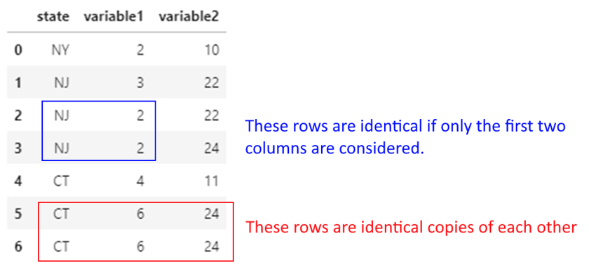
By default, all columns are considered, but you can limit the duplication detection to a subset of columns. If a subset of columns is used, the first observed value will be retained. This behavior can be changed by specifying keep = 'last'.

Let us consider an example. We create a toy dataframe as below:

Code

df = pd.DataFrame({'state': ['NY', 'NJ', 'NJ', 'NJ', 'CT', 'CT', 'CT'],
                  'variable1': [2, 3, 2, 2, 4, 6, 6],
                  'variable2': [10, 22, 22, 24, 11, 24, 24]})
df

	state	variable1	variable2
0	NY	2	10
1	NJ	3	22
2	NJ	2	22
3	NJ	2	24
4	CT	4	11
5	CT	6	24
6	CT	6	24

Note the below:

Code

## Dropping duplicates considering all columns

df.drop_duplicates()

	state	variable1	variable2
0	NY	2	10
1	NJ	3	22
2	NJ	2	22
3	NJ	2	24
4	CT	4	11
5	CT	6	24

Code

## Dropping duplicates considering only the first two columns.

## (Note which of the two NJ records was retained!)

df.drop_duplicates(['state', 'variable1'], keep='first')

	state	variable1	variable2
0	NY	2	10
1	NJ	3	22
2	NJ	2	22
4	CT	4	11
5	CT	6	24

9.16 Replacing Values

We often need to replace values in data. For example, we may know that 0 means the data is not available, and may wish to replace zeros with NaN.

Let us replace state names in our previous toy dataset with their full names.

We do this using df.replace({'NJ': 'New Jersey', 'NY': 'New York', 'CT': 'Connecticut’}).

Note that this affects the entire dataframe, so be careful to select the right column name if you want the replacement to occur in only one column!

Code

df.replace({'NJ': 'New Jersey', 'NY': 'New York', 'CT': 'Connecticut'})

	state	variable1	variable2
0	New York	2	10
1	New Jersey	3	22
2	New Jersey	2	22
3	New Jersey	2	24
4	Connecticut	4	11
5	Connecticut	6	24
6	Connecticut	6	24

9.17 Binning using Pandas `cut` Function

We often need to convert continuous variables into categories.

For example, reconsider our toy dataset. Consider variable1. Say we want anything 2 or lower to be labeled as Small, 2 to 4 as Medium, and 4 to 6 as Large.

We can do this as follows: pd.cut(df.variable1, [0, 2, 4, 6], labels = ["Small", "Medium", "Large"])

Consider variable1. Say we want anything 2 or lower to be labeled as Small, 2 to 4 as Medium, and 4 to 6 as Large.

We use the pd.cut function to create the bins, and assign them labels as below.

If no labels are specified, the mathematical notation for intervals will be used for the bins, ie [(0, 2] < (2, 4] < (4, 6]] ( ( means does not include, and [ means includes)

Code

df['NewColumn'] = pd.cut(df.variable1, [0, 2, 4, 6], labels = ["Small", "Medium", "Large"])
df

	state	variable1	variable2	NewColumn
0	NY	2	10	Small
1	NJ	3	22	Medium
2	NJ	2	22	Small
3	NJ	2	24	Small
4	CT	4	11	Medium
5	CT	6	24	Large
6	CT	6	24	Large

Code

df

	state	variable1	variable2	NewColumn
0	NY	2	10	Small
1	NJ	3	22	Medium
2	NJ	2	22	Small
3	NJ	2	24	Small
4	CT	4	11	Medium
5	CT	6	24	Large
6	CT	6	24	Large

Code

df['NewColumn'] = pd.cut(df.variable1, [0, 2, 4, 6])
df

	state	variable1	variable2	NewColumn
0	NY	2	10	(0, 2]
1	NJ	3	22	(2, 4]
2	NJ	2	22	(0, 2]
3	NJ	2	24	(0, 2]
4	CT	4	11	(2, 4]
5	CT	6	24	(4, 6]
6	CT	6	24	(4, 6]

9.18 Binning into Quantiles using `qcut`

Sometimes we may desire an equal number of observations in our bins.

In such cases, we can use quantiles as bins but then the intervals may not be equal (though the count of observations in each bin may be similar.

We can also specify arbitrary quantiles as bins.

In Pandas, use pd.qcut(df.variable1, number_of_quantiles) to achieve this.

Code

pd.qcut(df.variable1, 2)

0    (1.999, 3.0]
1    (1.999, 3.0]
2    (1.999, 3.0]
3    (1.999, 3.0]
4      (3.0, 6.0]
5      (3.0, 6.0]
6      (3.0, 6.0]
Name: variable1, dtype: category
Categories (2, interval[float64, right]): [(1.999, 3.0] < (3.0, 6.0]]

Code

pd.qcut(diamonds.price, 4)

0          (325.999, 950.0]
1          (325.999, 950.0]
2          (325.999, 950.0]
3          (325.999, 950.0]
4          (325.999, 950.0]
                ...        
27745    (5324.25, 18823.0]
27746    (5324.25, 18823.0]
27747    (5324.25, 18823.0]
27748    (5324.25, 18823.0]
27749    (5324.25, 18823.0]
Name: price, Length: 53940, dtype: category
Categories (4, interval[float64, right]): [(325.999, 950.0] < (950.0, 2401.0] < (2401.0, 5324.25] < (5324.25, 18823.0]]

Code

diamonds['quartiles']=pd.qcut(diamonds.price, 4)
diamonds['Price_Category']=pd.qcut(diamonds.price, 4, labels=['Economy','Affordable','Pricey','Expensive'])
diamonds.sample(8)

	price	carat	cut	color	clarity	depth	table	x	y	z	quartiles	Price_Category
44636	1608	0.58	Very Good	E	VS2	60.3	57.0	5.41	5.44	3.27	(950.0, 2401.0]	Affordable
27231	17597	1.70	Good	F	VS2	62.2	56.0	7.54	7.60	4.71	(5324.25, 18823.0]	Expensive
53017	2599	0.71	Good	G	VS2	64.2	58.0	5.59	5.62	3.60	(2401.0, 5324.25]	Pricey
29881	710	0.30	Very Good	D	VS2	60.3	60.0	4.28	4.31	2.59	(325.999, 950.0]	Economy
43150	1389	0.58	Ideal	H	SI1	61.9	59.0	5.33	5.36	3.31	(950.0, 2401.0]	Affordable
207	2778	0.52	Ideal	F	VVS1	61.3	55.0	5.19	5.22	3.19	(2401.0, 5324.25]	Pricey
15893	6354	1.01	Very Good	G	VVS2	61.3	61.0	6.32	6.47	3.92	(5324.25, 18823.0]	Expensive
29260	698	0.31	Premium	G	VS2	59.0	60.0	4.41	4.37	2.59	(325.999, 950.0]	Economy

Code

# ..combining pandas functions to get a list of the unique quartiles and price_category columns

diamonds[['quartiles', 'Price_Category']].drop_duplicates().sort_values(by='quartiles').reset_index()

	index	quartiles	Price_Category
0	0	(325.999, 950.0]	Economy
1	36691	(950.0, 2401.0]	Affordable
2	51735	(2401.0, 5324.25]	Pricey
3	12766	(5324.25, 18823.0]	Expensive

Code

# ..looking at counts in each category
diamonds.groupby(['quartiles', 'Price_Category'], observed=False).agg({"carat":"count"}).query('carat>0').rename({'carat':'Count of Diamonds'}, axis=1)

C:\Users\user\AppData\Local\Temp\ipykernel_17676\3774040384.py:2: FutureWarning: The default of observed=False is deprecated and will be changed to True in a future version of pandas. Pass observed=False to retain current behavior or observed=True to adopt the future default and silence this warning.
  diamonds.groupby(['quartiles', 'Price_Category']).agg({"carat":"count"}).query('carat>0').rename({'carat':'Count of Diamonds'}, axis=1)

		Count of Diamonds
quartiles	Price_Category
(325.999, 950.0]	Economy	13490
(950.0, 2401.0]	Affordable	13495
(2401.0, 5324.25]	Pricey	13470
(5324.25, 18823.0]	Expensive	13485

9.19 Select a random sample of data

Often, we need to look at a sample of the observations. df.head() and df.tail() produce the same records each time, and often it is good to look at other data.

df.sample(n) gives you a random set of n observations from the data.

Code

## Either a discrete number of rows,
diamonds.sample(3)

	price	carat	cut	color	clarity	depth	table	x	y	z	quartiles	Price_Category
14773	5946	1.01	Premium	G	VS2	59.0	61.0	6.62	6.56	3.89	(5324.25, 18823.0]	Expensive
14642	5913	1.20	Good	D	SI1	63.5	55.0	6.70	6.78	4.28	(5324.25, 18823.0]	Expensive
48244	1951	0.56	Good	E	VS1	59.8	61.0	5.35	5.36	3.20	(950.0, 2401.0]	Affordable

Code

## or a fraction of the total data
diamonds.sample(frac = 0.00015)

	price	carat	cut	color	clarity	depth	table	x	y	z	quartiles	Price_Category
38486	1031	0.42	Ideal	F	VS1	61.4	57.0	4.78	4.83	2.95	(950.0, 2401.0]	Affordable
23687	11746	1.51	Good	G	VS2	64.2	54.0	7.27	7.18	4.64	(5324.25, 18823.0]	Expensive
45832	1713	0.54	Ideal	E	VS2	62.8	55.0	5.21	5.24	3.28	(950.0, 2401.0]	Affordable
3947	3502	0.80	Premium	F	VS2	62.1	60.0	5.92	5.86	3.66	(2401.0, 5324.25]	Pricey
14828	5973	1.01	Very Good	E	SI1	63.1	57.0	6.40	6.37	4.03	(5324.25, 18823.0]	Expensive
25001	13530	1.52	Premium	F	VS2	59.4	60.0	7.61	7.50	4.49	(5324.25, 18823.0]	Expensive
6101	3975	0.91	Premium	G	SI1	61.8	60.0	6.21	6.18	3.83	(2401.0, 5324.25]	Pricey
3898	3489	0.89	Premium	H	VS1	60.5	59.0	6.22	6.17	3.75	(2401.0, 5324.25]	Pricey

9.20 String operations with Pandas

We often have to combine text data, split it, find certain types of text, and perform various other functions on strings.

String munging operations often take up a lot of time when cleaning data.

Pandas offers a number of methods to perform string operations – refer list to the right.

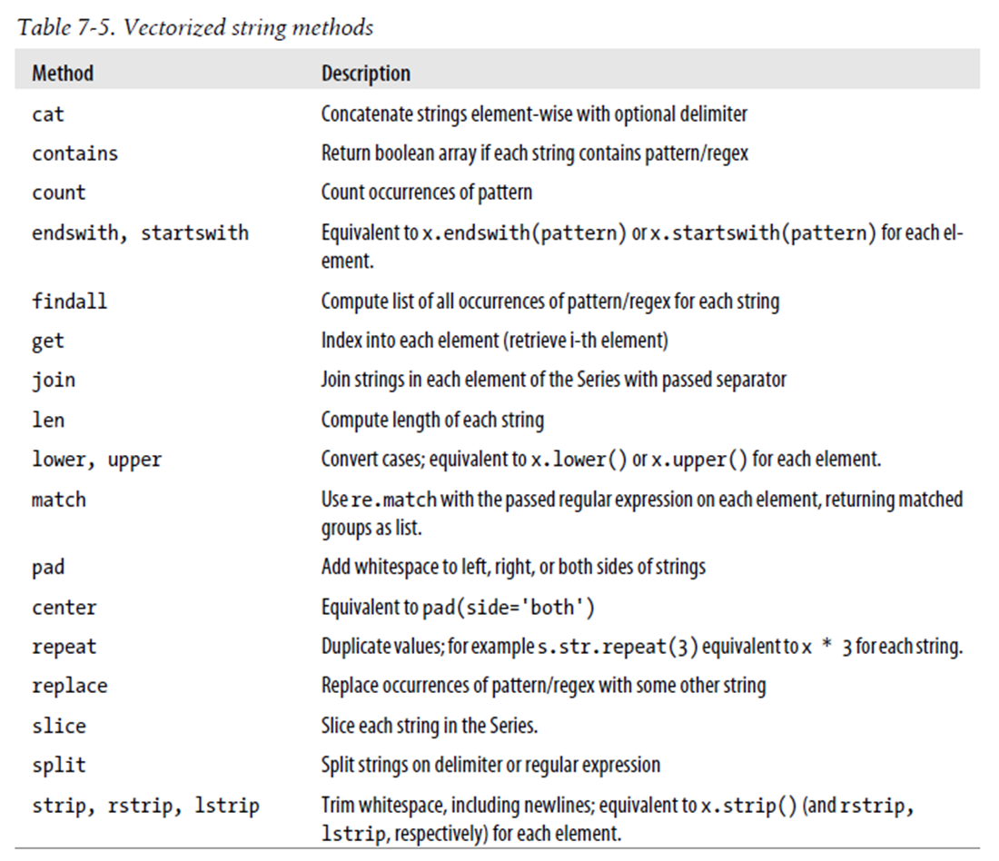
Source: Python for Data Analysis, Wes McKinney

9.21 Value Counts

Code

mtcars

	mpg	cyl	disp	hp	drat	wt	qsec	vs	am	gear	carb
rownames
Mazda RX4	21.0	6	160.0	110	3.90	2.620	16.46	0	1	4	4
Mazda RX4 Wag	21.0	6	160.0	110	3.90	2.875	17.02	0	1	4	4
Datsun 710	22.8	4	108.0	93	3.85	2.320	18.61	1	1	4	1
Hornet 4 Drive	21.4	6	258.0	110	3.08	3.215	19.44	1	0	3	1
Hornet Sportabout	18.7	8	360.0	175	3.15	3.440	17.02	0	0	3	2
Valiant	18.1	6	225.0	105	2.76	3.460	20.22	1	0	3	1
Duster 360	14.3	8	360.0	245	3.21	3.570	15.84	0	0	3	4
Merc 240D	24.4	4	146.7	62	3.69	3.190	20.00	1	0	4	2
Merc 230	22.8	4	140.8	95	3.92	3.150	22.90	1	0	4	2
Merc 280	19.2	6	167.6	123	3.92	3.440	18.30	1	0	4	4
Merc 280C	17.8	6	167.6	123	3.92	3.440	18.90	1	0	4	4
Merc 450SE	16.4	8	275.8	180	3.07	4.070	17.40	0	0	3	3
Merc 450SL	17.3	8	275.8	180	3.07	3.730	17.60	0	0	3	3
Merc 450SLC	15.2	8	275.8	180	3.07	3.780	18.00	0	0	3	3
Cadillac Fleetwood	10.4	8	472.0	205	2.93	5.250	17.98	0	0	3	4
Lincoln Continental	10.4	8	460.0	215	3.00	5.424	17.82	0	0	3	4
Chrysler Imperial	14.7	8	440.0	230	3.23	5.345	17.42	0	0	3	4
Fiat 128	32.4	4	78.7	66	4.08	2.200	19.47	1	1	4	1
Honda Civic	30.4	4	75.7	52	4.93	1.615	18.52	1	1	4	2
Toyota Corolla	33.9	4	71.1	65	4.22	1.835	19.90	1	1	4	1
Toyota Corona	21.5	4	120.1	97	3.70	2.465	20.01	1	0	3	1
Dodge Challenger	15.5	8	318.0	150	2.76	3.520	16.87	0	0	3	2
AMC Javelin	15.2	8	304.0	150	3.15	3.435	17.30	0	0	3	2
Camaro Z28	13.3	8	350.0	245	3.73	3.840	15.41	0	0	3	4
Pontiac Firebird	19.2	8	400.0	175	3.08	3.845	17.05	0	0	3	2
Fiat X1-9	27.3	4	79.0	66	4.08	1.935	18.90	1	1	4	1
Porsche 914-2	26.0	4	120.3	91	4.43	2.140	16.70	0	1	5	2
Lotus Europa	30.4	4	95.1	113	3.77	1.513	16.90	1	1	5	2
Ford Pantera L	15.8	8	351.0	264	4.22	3.170	14.50	0	1	5	4
Ferrari Dino	19.7	6	145.0	175	3.62	2.770	15.50	0	1	5	6
Maserati Bora	15.0	8	301.0	335	3.54	3.570	14.60	0	1	5	8
Volvo 142E	21.4	4	121.0	109	4.11	2.780	18.60	1	1	4	2

Code

## value_counts provide the frequency for categorical variables
mtcars.cyl.value_counts()

cyl
8    14
4    11
6     7
Name: count, dtype: int64

Code

## ...and we can get percentages instead too
mtcars.cyl.value_counts(normalize=True)

cyl
8    0.43750
4    0.34375
6    0.21875
Name: proportion, dtype: float64

Code

# Just checking what range(60,64) returns

list(range(60,64))

[60, 61, 62, 63]

Code

diamonds.depth.describe()

count    53940.000000
mean        61.749405
std          1.432621
min         43.000000
25%         61.000000
50%         61.800000
75%         62.500000
max         79.000000
Name: depth, dtype: float64

Code

## We can specify bins for numerical variables
# Below, we are saying give us value counts for 60-61, 61-62, 62-63.

diamonds = sns.load_dataset("diamonds")

diamonds.depth.value_counts(bins = range(60,64))

(61.0, 62.0]      17945
(62.0, 63.0]      15348
(59.999, 61.0]     8451
Name: count, dtype: int64

Code

# Let us create a random vehicle crash dataframe with three columns showing
# city, cause of crash, and the dollar loss from the accident.
# Some of the values are missing, and indicated as a NaN (we create Nan
# values using np.nan)

df = pd.DataFrame(data = {'city': ['NYC', np.nan, 'Boston', 'Boston', 
                                   'WashingtonDC', np.nan, 'Boston', 
                                   'NYC', 'Boston', 'NYC'],
                         'cause': ['distracted', 'drowsy', 'drowsy', 
                                   np.nan, 'drunk', 'distracted', 
                                   'distracted', np.nan, np.nan, 'drunk'],
                         'dollar_loss': [8194, 4033, 9739, 4876, 4421, 
                                         6094, 5080, 2909, 9712, 2450]})

df

	city	cause	dollar_loss
0	NYC	distracted	8194
1	NaN	drowsy	4033
2	Boston	drowsy	9739
3	Boston	NaN	4876
4	WashingtonDC	drunk	4421
5	NaN	distracted	6094
6	Boston	distracted	5080
7	NYC	NaN	2909
8	Boston	NaN	9712
9	NYC	drunk	2450

Code

# Let us check the value_counts by city
# By default, missing values are ignored.
# So you don't see the NaNs.
# You can address it by setting dropna = False, as in the next cell

df.city.value_counts()

city
Boston          4
NYC             3
WashingtonDC    1
Name: count, dtype: int64

Code

df.city.value_counts(dropna = False)

city
Boston          4
NYC             3
NaN             2
WashingtonDC    1
Name: count, dtype: int64

Code

# Instead of counts, you can ask for percentages (expressed as a decimal)

df.city.value_counts(dropna = False, normalize = True)

city
Boston          0.4
NYC             0.3
NaN             0.2
WashingtonDC    0.1
Name: proportion, dtype: float64

Code

# Sometimes, you may use the cumulative sum function to get 
# totals upto that value.  Try to run the cell to understand what it does.

df.city.value_counts().cumsum()

city
Boston          4
NYC             7
WashingtonDC    8
Name: count, dtype: int64

Code

df.city.value_counts(dropna = False, normalize = True).cumsum()

city
Boston          0.4
NYC             0.7
NaN             0.9
WashingtonDC    1.0
Name: proportion, dtype: float64

9.22 Extract unique values

9.22.1 Fuzzy String Matching

Real-world data often has slight variations in string values (e.g., “New York” vs “new york” vs “NY”). The thefuzz library handles this efficiently:

# pip install thefuzz
from thefuzz import fuzz, process

fuzz.ratio("New York", "new york")          # 89 — case insensitive similarity
fuzz.partial_ratio("NYC", "New York City")  # 100 — partial match

# Find best match from a candidate list
process.extractOne("New Yrok", ["New York", "New Jersey", "Newark"])
# Returns: ("New York", 91, 0)

This is invaluable when joining datasets from different sources where category labels do not match exactly.

Code

diamonds.cut.unique()
## You can put `tolist()` at the end to get a cleaner output, or enclose everything in `list`.

['Ideal', 'Premium', 'Good', 'Very Good', 'Fair']
Categories (5, object): ['Ideal', 'Premium', 'Very Good', 'Good', 'Fair']

9.23 Groupby

groupby and rename use as parameters the dict format, which is curly brackets, and key : value, each within quotes.

For example, {"old_colname" : "new_colname", "old_colname2" : "new_colname2"}

Code

mydf = diamonds.groupby('cut', observed=True)
summ = mydf.agg({"price": "sum", "clarity": "count", "table": "mean"}) 
summ

	price	clarity	table
cut
Ideal	74513487	21551	55.951668
Premium	63221498	13791	58.746095
Very Good	48107623	12082	57.956150
Good	19275009	4906	58.694639
Fair	7017600	1610	59.053789

Code

## Alternatively, everything could be combined together:
diamonds.groupby('cut', observed=True).agg({"price": "sum", "clarity": "count", "table": "mean"})

	price	clarity	table
cut
Ideal	74513487	21551	55.951668
Premium	63221498	13791	58.746095
Very Good	48107623	12082	57.956150
Good	19275009	4906	58.694639
Fair	7017600	1610	59.053789

Code

## Or, groupby two variables:
diamonds.groupby(['cut', 'color'], observed=True).agg({"price": "sum", "clarity": "count", "table": "mean"})

		price	clarity	table
cut	color
Ideal	D	7450854	2834	55.965632
	E	10138238	3903	55.967461
	F	12912518	3826	55.924203
	G	18171930	4884	55.902375
	H	12115278	3115	55.965843
	I	9317974	2093	56.021357
	J	4406695	896	56.012612
Premium	D	5820962	1603	58.718964
	E	8270443	2337	58.779461
	F	10081319	2331	58.679279
	G	13160170	2924	58.702360
	H	12311428	2360	58.792034
	I	8491146	1428	58.771849
	J	5086030	808	58.874752
Very Good	D	5250817	1513	58.041309
	E	7715165	2400	58.038875
	F	8177367	2164	57.848429
	G	8903461	2299	57.784428
	H	8272552	1824	57.903015
	I	6328079	1204	58.105150
	J	3460182	678	58.277729
Good	D	2254363	662	58.541541
	E	3194260	933	58.779957
	F	3177637	909	58.910891
	G	3591553	871	58.471986
	H	3001931	702	58.611111
	I	2650994	522	58.773946
	J	1404271	307	58.813029
Fair	D	699443	163	58.969325
	E	824838	224	59.364732
	F	1194025	312	59.453205
	G	1331126	314	58.773248
	H	1556112	303	58.696370
	I	819953	175	59.237143
	J	592103	119	58.917647

9.23.1 `rename` columns with Groupby

9.23.2 Named Aggregations (Preferred Style)

Pandas 0.25+ introduced named aggregations, which produce cleaner output and are more readable:

# Old style -- column names can be ambiguous:
df.groupby("cut").agg({"price": ["mean", "sum"], "carat": "count"})

# New style -- named aggregation (pandas 0.25+):
df.groupby("cut").agg(
    avg_price=("price", "mean"),
    total_price=("price", "sum"),
    diamond_count=("carat", "count")
)

Named aggregation is preferred in production code because output column names are explicit and deterministic.

Code

## We continue the above examples to rename the aggregated columns we created using groupby

diamonds.groupby('cut', observed=True).agg({"price": "sum", 
                             "clarity": "count"}).rename(columns = {"price": "total_price", "clarity": "diamond_count"})

	total_price	diamond_count
cut
Ideal	74513487	21551
Premium	63221498	13791
Very Good	48107623	12082
Good	19275009	4906
Fair	7017600	1610

9.24 Joining Data with Merge

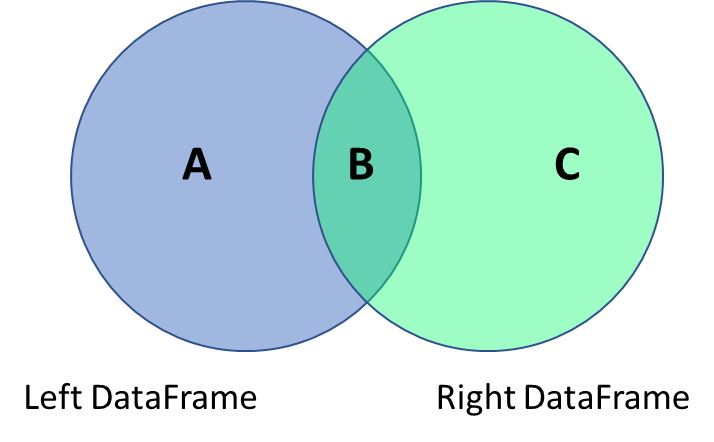
The data analyst often has to combine data frames much in the same way as database join operations work, which requires connecting two tables based on a reference field.

(joins of all types are discussed here: https://pandas.pydata.org/pandas-docs/stable/user_guide/merging.htmlhttps://pandas.pydata.org/pandas-docs/stable/user_guide/merging.html)

Outer Join = A + B + C (keep everything)
Inner Join = B (keep only the intersection)
Left Join = A + B (keep all from the left)
Right Join = B + C (keep all from the right)

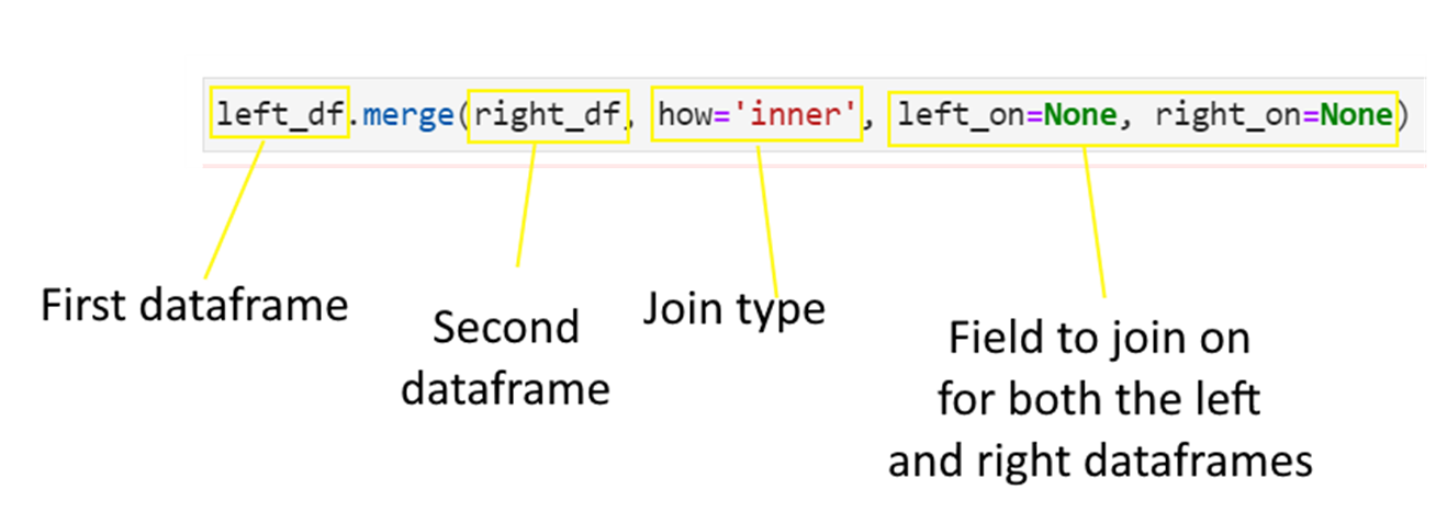
You can join data using the pandas merge function.

Consider the below data frames. The first one is the left data frame, and the second one is the right data frame.

Next consider the four types of joins - left, right, inner and outer.

Code

## Left data frame

np.random.seed(2)
n = 5
df = pd.DataFrame(
    {'state': list(np.random.choice(["New York", "Florida", "California"], size=(n))), 
     'gender': list(np.random.choice(["Male", "Female"], size=(n), p=[.4, .6])),
     'housing': list(np.random.choice(["Rent", "Own"], size=(n))),     
     'height': list(np.random.randint(140,200,n))
     })

Code

## Left data frame

df

	state	gender	housing	height
0	New York	Female	Own	177
1	Florida	Male	Rent	179
2	New York	Male	Rent	143
3	California	Female	Rent	178
4	California	Male	Rent	144

Code

## Right data frame

df_rent = pd.DataFrame(
          {'state': ["Connecticut", "Florida", "California"],
           'avg_rent': [3500, 2200, 4500]})

Code

## Right data frame

df_rent

	state	avg_rent
0	Connecticut	3500
1	Florida	2200
2	California	4500

9.24.1 Left Join

Code

df.merge(df_rent, how = 'left' , 
         left_on = 'state', right_on = 'state')

	state	gender	housing	height	avg_rent
0	New York	Female	Own	177	NaN
1	Florida	Male	Rent	179	2200.0
2	New York	Male	Rent	143	NaN
3	California	Female	Rent	178	4500.0
4	California	Male	Rent	144	4500.0

9.24.2 Right Join

Code

df.merge(df_rent, how = 'right' , 
         left_on = 'state', right_on = 'state')

	state	gender	housing	height	avg_rent
0	Connecticut	NaN	NaN	NaN	3500
1	Florida	Male	Rent	179.0	2200
2	California	Female	Rent	178.0	4500
3	California	Male	Rent	144.0	4500

9.24.3 Inner Join

Code

df.merge(df_rent, how = 'inner' , 
         left_on = 'state', right_on = 'state')

	state	gender	housing	height	avg_rent
0	Florida	Male	Rent	179	2200
1	California	Female	Rent	178	4500
2	California	Male	Rent	144	4500

9.24.4 Outer Join

Code

df.merge(df_rent, how = 'outer' , 
         left_on = 'state', right_on = 'state')

	state	gender	housing	height	avg_rent
0	California	Female	Rent	178.0	4500.0
1	California	Male	Rent	144.0	4500.0
2	Connecticut	NaN	NaN	NaN	3500.0
3	Florida	Male	Rent	179.0	2200.0
4	New York	Female	Own	177.0	NaN
5	New York	Male	Rent	143.0	NaN

9.24.5 Cross Join

Join everything with everything!

Code

df.merge(df_rent, how = 'cross')

	state_x	gender	housing	height	state_y	avg_rent
0	New York	Female	Own	177	Connecticut	3500
1	New York	Female	Own	177	Florida	2200
2	New York	Female	Own	177	California	4500
3	Florida	Male	Rent	179	Connecticut	3500
4	Florida	Male	Rent	179	Florida	2200
5	Florida	Male	Rent	179	California	4500
6	New York	Male	Rent	143	Connecticut	3500
7	New York	Male	Rent	143	Florida	2200
8	New York	Male	Rent	143	California	4500
9	California	Female	Rent	178	Connecticut	3500
10	California	Female	Rent	178	Florida	2200
11	California	Female	Rent	178	California	4500
12	California	Male	Rent	144	Connecticut	3500
13	California	Male	Rent	144	Florida	2200
14	California	Male	Rent	144	California	4500

9.25 Concatenation

Sometimes we need to simply combine datasets without any fancy operations.

Imagine you have 3 files, each for a different month, and you need to stack them vertically one after the other.

Occasionally, you may need to stack datasets horizontally, ie right next to each other. For example, imagine you have 2 files, one with names and ages, and the other with names and income. You may just want to ‘stack’ the data next to each other.

As a common operation, this can be done with Pandas’s concat() command.

We use the same df and df_rent dataframes as in the prior slide to illustrate how pd.concat works.

Code

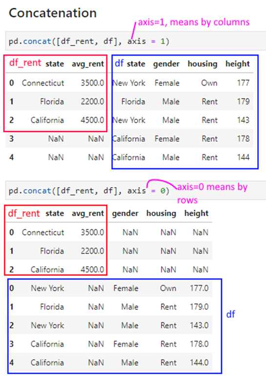
pd.concat([df_rent, df], axis = 1)

	state	avg_rent	state	gender	housing	height
0	Connecticut	3500.0	New York	Female	Own	177
1	Florida	2200.0	Florida	Male	Rent	179
2	California	4500.0	New York	Male	Rent	143
3	NaN	NaN	California	Female	Rent	178
4	NaN	NaN	California	Male	Rent	144

Code

pd.concat([df_rent, df], axis = 0)

	state	avg_rent	gender	housing	height
0	Connecticut	3500.0	NaN	NaN	NaN
1	Florida	2200.0	NaN	NaN	NaN
2	California	4500.0	NaN	NaN	NaN
0	New York	NaN	Female	Own	177.0
1	Florida	NaN	Male	Rent	179.0
2	New York	NaN	Male	Rent	143.0
3	California	NaN	Female	Rent	178.0
4	California	NaN	Male	Rent	144.0

9.25.1 Concatenation example

We load the penguins dataset.

Code

# Load the penguins dataset

df = sns.load_dataset('penguins')
df

	species	island	bill_length_mm	bill_depth_mm	flipper_length_mm	body_mass_g	sex
0	Adelie	Torgersen	39.1	18.7	181.0	3750.0	Male
1	Adelie	Torgersen	39.5	17.4	186.0	3800.0	Female
2	Adelie	Torgersen	40.3	18.0	195.0	3250.0	Female
3	Adelie	Torgersen	NaN	NaN	NaN	NaN	NaN
4	Adelie	Torgersen	36.7	19.3	193.0	3450.0	Female
...	...	...	...	...	...	...	...
339	Gentoo	Biscoe	NaN	NaN	NaN	NaN	NaN
340	Gentoo	Biscoe	46.8	14.3	215.0	4850.0	Female
341	Gentoo	Biscoe	50.4	15.7	222.0	5750.0	Male
342	Gentoo	Biscoe	45.2	14.8	212.0	5200.0	Female
343	Gentoo	Biscoe	49.9	16.1	213.0	5400.0	Male

344 rows × 7 columns

Code

df1 = df.sample(6).reset_index(drop=True)
df2 = df.sample(4).reset_index(drop=True)

Code

df1

	species	island	bill_length_mm	bill_depth_mm	flipper_length_mm	body_mass_g	sex
0	Gentoo	Biscoe	45.2	15.8	215.0	5300.0	Male
1	Adelie	Biscoe	37.9	18.6	172.0	3150.0	Female
2	Adelie	Biscoe	37.8	18.3	174.0	3400.0	Female
3	Adelie	Dream	40.6	17.2	187.0	3475.0	Male
4	Chinstrap	Dream	50.1	17.9	190.0	3400.0	Female
5	Gentoo	Biscoe	46.5	13.5	210.0	4550.0	Female

Code

df1.columns

Index(['species', 'island', 'bill_length_mm', 'bill_depth_mm',
       'flipper_length_mm', 'body_mass_g', 'sex'],
      dtype='object')

Code

df1 = df1[['bill_length_mm', 'bill_depth_mm','body_mass_g', 'sex','flipper_length_mm', ]]
df1

	bill_length_mm	bill_depth_mm	body_mass_g	sex	flipper_length_mm
0	45.2	15.8	5300.0	Male	215.0
1	37.9	18.6	3150.0	Female	172.0
2	37.8	18.3	3400.0	Female	174.0
3	40.6	17.2	3475.0	Male	187.0
4	50.1	17.9	3400.0	Female	190.0
5	46.5	13.5	4550.0	Female	210.0

Code

df2

	species	island	bill_length_mm	bill_depth_mm	flipper_length_mm	body_mass_g	sex
0	Gentoo	Biscoe	46.4	15.6	221.0	5000.0	Male
1	Gentoo	Biscoe	48.4	14.4	203.0	4625.0	Female
2	Gentoo	Biscoe	49.0	16.1	216.0	5550.0	Male
3	Adelie	Torgersen	35.9	16.6	190.0	3050.0	Female

Code

pd.concat([df1,df2], axis=0)

	bill_length_mm	bill_depth_mm	body_mass_g	sex	flipper_length_mm	species	island
0	45.2	15.8	5300.0	Male	215.0	NaN	NaN
1	37.9	18.6	3150.0	Female	172.0	NaN	NaN
2	37.8	18.3	3400.0	Female	174.0	NaN	NaN
3	40.6	17.2	3475.0	Male	187.0	NaN	NaN
4	50.1	17.9	3400.0	Female	190.0	NaN	NaN
5	46.5	13.5	4550.0	Female	210.0	NaN	NaN
0	46.4	15.6	5000.0	Male	221.0	Gentoo	Biscoe
1	48.4	14.4	4625.0	Female	203.0	Gentoo	Biscoe
2	49.0	16.1	5550.0	Male	216.0	Gentoo	Biscoe
3	35.9	16.6	3050.0	Female	190.0	Adelie	Torgersen

Code

pd.concat([df1,df2], axis=0)

	species	island	bill_length_mm	bill_depth_mm	flipper_length_mm	body_mass_g	sex
0	Gentoo	Biscoe	45.2	15.8	215.0	5300.0	Male
1	Adelie	Biscoe	37.9	18.6	172.0	3150.0	Female
2	Adelie	Biscoe	37.8	18.3	174.0	3400.0	Female
3	Adelie	Dream	40.6	17.2	187.0	3475.0	Male
4	Chinstrap	Dream	50.1	17.9	190.0	3400.0	Female
5	Gentoo	Biscoe	46.5	13.5	210.0	4550.0	Female
0	Gentoo	Biscoe	46.4	15.6	221.0	5000.0	Male
1	Gentoo	Biscoe	48.4	14.4	203.0	4625.0	Female
2	Gentoo	Biscoe	49.0	16.1	216.0	5550.0	Male
3	Adelie	Torgersen	35.9	16.6	190.0	3050.0	Female

Code

pd.concat([df1,df2], axis=1)

	species	island	bill_length_mm	bill_depth_mm	flipper_length_mm	body_mass_g	sex	species	island	bill_length_mm	bill_depth_mm	flipper_length_mm	body_mass_g	sex
0	Gentoo	Biscoe	45.2	15.8	215.0	5300.0	Male	Gentoo	Biscoe	46.4	15.6	221.0	5000.0	Male
1	Adelie	Biscoe	37.9	18.6	172.0	3150.0	Female	Gentoo	Biscoe	48.4	14.4	203.0	4625.0	Female
2	Adelie	Biscoe	37.8	18.3	174.0	3400.0	Female	Gentoo	Biscoe	49.0	16.1	216.0	5550.0	Male
3	Adelie	Dream	40.6	17.2	187.0	3475.0	Male	Adelie	Torgersen	35.9	16.6	190.0	3050.0	Female
4	Chinstrap	Dream	50.1	17.9	190.0	3400.0	Female	NaN	NaN	NaN	NaN	NaN	NaN	NaN
5	Gentoo	Biscoe	46.5	13.5	210.0	4550.0	Female	NaN	NaN	NaN	NaN	NaN	NaN	NaN

Code

df2.index = [3,4,5,6]

Code

pd.concat([df1,df2], axis=0)

	species	island	bill_length_mm	bill_depth_mm	flipper_length_mm	body_mass_g	sex
0	Gentoo	Biscoe	45.2	15.8	215.0	5300.0	Male
1	Adelie	Biscoe	37.9	18.6	172.0	3150.0	Female
2	Adelie	Biscoe	37.8	18.3	174.0	3400.0	Female
3	Adelie	Dream	40.6	17.2	187.0	3475.0	Male
4	Chinstrap	Dream	50.1	17.9	190.0	3400.0	Female
5	Gentoo	Biscoe	46.5	13.5	210.0	4550.0	Female
3	Gentoo	Biscoe	46.4	15.6	221.0	5000.0	Male
4	Gentoo	Biscoe	48.4	14.4	203.0	4625.0	Female
5	Gentoo	Biscoe	49.0	16.1	216.0	5550.0	Male
6	Adelie	Torgersen	35.9	16.6	190.0	3050.0	Female

Code

pd.concat([df1,df2], axis=1)

	species	island	bill_length_mm	bill_depth_mm	flipper_length_mm	body_mass_g	sex	species	island	bill_length_mm	bill_depth_mm	flipper_length_mm	body_mass_g	sex
0	Gentoo	Biscoe	45.2	15.8	215.0	5300.0	Male	NaN	NaN	NaN	NaN	NaN	NaN	NaN
1	Adelie	Biscoe	37.9	18.6	172.0	3150.0	Female	NaN	NaN	NaN	NaN	NaN	NaN	NaN
2	Adelie	Biscoe	37.8	18.3	174.0	3400.0	Female	NaN	NaN	NaN	NaN	NaN	NaN	NaN
3	Adelie	Dream	40.6	17.2	187.0	3475.0	Male	Gentoo	Biscoe	46.4	15.6	221.0	5000.0	Male
4	Chinstrap	Dream	50.1	17.9	190.0	3400.0	Female	Gentoo	Biscoe	48.4	14.4	203.0	4625.0	Female
5	Gentoo	Biscoe	46.5	13.5	210.0	4550.0	Female	Gentoo	Biscoe	49.0	16.1	216.0	5550.0	Male
6	NaN	NaN	NaN	NaN	NaN	NaN	NaN	Adelie	Torgersen	35.9	16.6	190.0	3050.0	Female

Code

# Notice above dataframe has columns with identical names
# For example,the column bill_depth_mm appears twice.
# If we try to select that column, all columns with that name are listed

temp = pd.concat([df1,df2], axis=1)
temp[['bill_depth_mm']]

	bill_depth_mm	bill_depth_mm
0	15.8	NaN
1	18.6	NaN
2	18.3	NaN
3	17.2	15.6
4	17.9	14.4
5	13.5	16.1
6	NaN	16.6

9.26 Dealing with Missing Values

Missing data takes one of two forms.
1. Entire rows of data may be missing: In such situations, you will need to think about if the remaining data set is still valuable.
- Consider if you can assess how much data is missing. If only a small portion of the data is missing, say 10%, then you may still be able to use it for meaningful analytics.
- Consider why the data is missing. If the absent data is missing at random, what you have available may still be a representative sample.
- Consider if you can re-acquire the data, or address the underlying problems and wait to collect the complete dataset.
2. Some values may be missing in the data, while others are present.
- We can remove the rows that have missing values.
- We can replace the missing values with a static default (eg, the mean, or the median).
- We can try to compute the values in a more structured way.

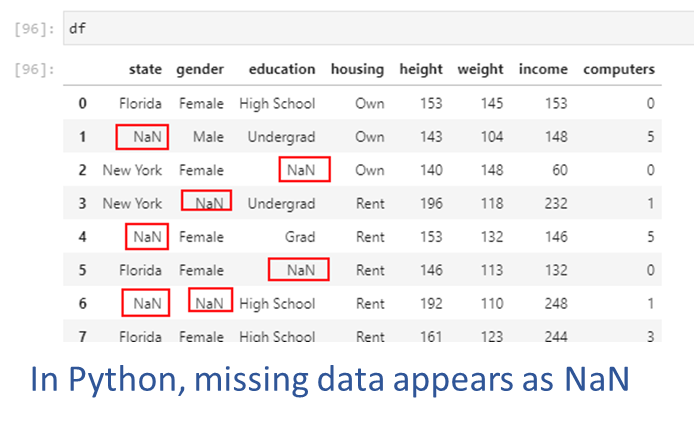
An example of missing data appears in the picture below. Next, we will create this dataset and artifically insert some missing values.

Code

YouTubeVideo('106wMohSma8', width=672, height=378)

Code

## We create a random dataset

np.random.seed(1)
n = 5
df = pd.DataFrame(
    {'state': list(np.random.choice(["New York", "Florida", "California"], size=(n))), 
     'gender': list(np.random.choice(["Male", "Female"], size=(n), p=[.4, .6])),
     'housing': list(np.random.choice(["Rent", "Own"], size=(n))),    
     'height': list(np.random.randint(140,200,n))
     })

Code

## Now we loop through the data and replace a quarter of the values with NaN (`np.nan`)

for row in range(df.shape[0]):
    for col in range(df.shape[1]):
        if np.random.uniform() < 0.25:
            df.iloc[row,col] = np.nan

Code

## Notice the `NaN` values inserted  
df

	state	gender	housing	height
0	Florida	Male	Rent	160.0
1	New York	Male	Rent	151.0
2	NaN	Male	Rent	182.0
3	Florida	Male	NaN	168.0
4	Florida	Male	Rent	NaN

9.26.1 Understanding the extent of missing values

We can count the number of null values, by rows as well as columns.

In pandas, it is easy to identify null values using df.isna(). While this provides us a series of True/False Booleans, we can use the sum() command to get the total count of nulls as Booleans are also considered equal to 1 and 0 (for True and False respectively).

Using the axis parameter, we can specify whether to count missing values by rows (axis = 1) or by columns (axis = 0, the default).

Count of nulls for each column: df.isna().sum(axis=0)
Count of nulls for each row: df.isna().sum(axis=1)

Code

## Count missing values - by columns

df.isna().sum(axis=0)

state      1
gender     0
housing    1
height     1
dtype: int64

Code

## Count missing values - by rows

df.isna().sum(axis=1)

0    0
1    0
2    1
3    1
4    1
dtype: int64

Code

## Count missing values - by columns, sorted

df.isna().sum(axis=0).sort_values(ascending=False)

state      1
housing    1
height     1
gender     0
dtype: int64

Code

df.isna().sum(axis=1).sort_values(ascending=False)

2    1
3    1
4    1
0    0
1    0
dtype: int64

9.26.2 How to think about missing values

Sometimes, entire rows/observations or columns/features data may be missing in the data (for example, you discover that you are missing data for a city, person, year etc). If the data is not there in the first place, there is no easy programmatic way to discover the omission. You may find out about it only accidentally, or through your exploratory data analysis.

In such situations, you will need to think about if the remaining data set is still valuable.
- Consider if you can assess how much data is missing. If only a small portion of the data is missing, say 10%, then you may still be able to use it for meaningful analytics.
- Consider why the data is missing. If the absent data is missing at random, what you have available may still be a representative sample.
- Consider if you can re-acquire the data, or address the underlying problems and wait to collect the complete dataset.

Approaches
When some values in the data are missing:
1. Drop rows with nulls: If data is missing at random, and the remaining data is sufficient for us to build generalizable analytics and models.
- If data is not missing at random, and rows with missing data are dropped, this can introduce bias into our models.
2. Drop features/columns with nulls: Features that have a great deal of data missing at random can often be dropped without affecting analytical usefulness.
3. Replace with a static default: Using a summary statistic, eg mean or median, is often an easy way to replace missing values.
4. Impute missing values using more advanced methods.

9.26.2.1 Drop Missing Values

The simplest approach is to drop the rows that have a missing value. This will leave only the rows that are fully populated.

Pandas offers the function dropna() to remove rows with missing values.

You can control which rows are deleted:

Set a threshold n – at least n values must be missing before the row is dropped
Any or All – whether all values should be missing, or any missing values.

9.26.2.1.1 Drop rows with missing values

Code

df

	state	gender	housing	height
0	Florida	Male	Rent	160.0
1	New York	Male	Rent	151.0
2	NaN	Male	Rent	182.0
3	Florida	Male	NaN	168.0
4	Florida	Male	Rent	NaN

Code

df.dropna()

	state	gender	housing	height
0	Florida	Male	Rent	160.0
1	New York	Male	Rent	151.0

9.26.2.1.2 Drop columns with missing values

Very similar approach as for rows, except the axis along which we evaluate deletion is vertical instead of horizontal.

Any columns that have a missing value are deleted.

Code

df.dropna(axis = 1)

	gender
0	Male
1	Male
2	Male
3	Male
4	Male

Code

df

	state	gender	housing	height
0	Florida	Male	Rent	160.0
1	New York	Male	Rent	151.0
2	NaN	Male	Rent	182.0
3	Florida	Male	NaN	168.0
4	Florida	Male	Rent	NaN

9.26.2.2 Fill Missing Data

Dropping rows or columns that have missing data may not always be a feasible strategy as the remainder of the dataset may become too small.

Another reason is that we may not want to throw away all the other known information just because one data point for an observation or a feature is not known.

If the data is not missing at random (for example, one sensor in the data collection apparatus was malfunctioning) and all the NaN values relate to a particular type of observation, we will introduce bias into any analytics we perform.

A viable approach in such cases may be to replace the missing values with an estimate, such as the mean, the median, or the most frequent value.

Using pd.fillna(), we can fill any holes in the data in a number of ways. With df.fillna(constant), we can replace all NaN values with a constant we specify. However, if NaNs appear in multiple columns, we may need to specify a different constant for each column.

With pd.fillna(data.mean()), we can replace NaNs with the mean, and similarly for median and other calculated measures.

Code

## Fill missing values across the entire dataframe

df.fillna('Connecticut')

	state	gender	housing	height
0	Florida	Male	Rent	160.0
1	New York	Male	Rent	151.0
2	Connecticut	Male	Rent	182.0
3	Florida	Male	Connecticut	168.0
4	Florida	Male	Rent	Connecticut

Code

## Fill missing values in only a single column

df.fillna({'housing': 'Connecticut'}, inplace=True)
df

	species	island	bill_length_mm	bill_depth_mm	flipper_length_mm	body_mass_g	sex
0	Adelie	Torgersen	39.1	18.7	181.0	3750.0	Male
1	Adelie	Torgersen	39.5	17.4	186.0	3800.0	Female
2	Adelie	Torgersen	40.3	18.0	195.0	3250.0	Female
3	Adelie	Torgersen	NaN	NaN	NaN	NaN	NaN
4	Adelie	Torgersen	36.7	19.3	193.0	3450.0	Female
...	...	...	...	...	...	...	...
339	Gentoo	Biscoe	NaN	NaN	NaN	NaN	NaN
340	Gentoo	Biscoe	46.8	14.3	215.0	4850.0	Female
341	Gentoo	Biscoe	50.4	15.7	222.0	5750.0	Male
342	Gentoo	Biscoe	45.2	14.8	212.0	5200.0	Female
343	Gentoo	Biscoe	49.9	16.1	213.0	5400.0	Male

344 rows × 7 columns

9.26.3 Forward and Backward Fill

For time series data, we might like to use forward-fill (also called ‘last-observation-carried-forward’, or locf), and backward-fill (opposite of locf).

df.ffill: propagate last valid observation forward to next valid
df.bfill: use next valid observation to fill gap.

Code

## Let us make some of the height numbers NaN
df.loc[[0,3], 'height'] = np.nan

Code

df

	state	gender	housing	height
0	Florida	Male	Rent	NaN
1	New York	Male	Rent	151.0
2	Connecticut	Male	Rent	182.0
3	Florida	Male	NaN	NaN
4	Florida	Male	Rent	NaN

Code

# Forward fill
df.ffill()

	state	gender	housing	height
0	Florida	Male	Rent	NaN
1	New York	Male	Rent	151.0
2	Connecticut	Male	Rent	182.0
3	Florida	Male	Rent	182.0
4	Florida	Male	Rent	182.0

Code

# Backward fill
df.bfill()

	state	gender	housing	height
0	Florida	Male	Rent	151.0
1	New York	Male	Rent	151.0
2	Connecticut	Male	Rent	182.0
3	Florida	Male	Rent	NaN
4	Florida	Male	Rent	NaN

Code

# We load some data on sales of independent winemakers
import pmdarima
df = pd.DataFrame(pmdarima.datasets.load_wineind(as_series = True), columns=['sales'])
df

	sales
Jan 1980	15136.0
Feb 1980	16733.0
Mar 1980	20016.0
Apr 1980	17708.0
May 1980	18019.0
...	...
Apr 1994	26323.0
May 1994	23779.0
Jun 1994	27549.0
Jul 1994	29660.0
Aug 1994	23356.0

176 rows × 1 columns

Code

## Now we loop through the data and replace a quarter of the values with NaN (`np.nan`)

for row in range(df.shape[0]):
    for col in range(df.shape[1]):
        if np.random.uniform() < 0.5:
            df.iloc[row,col] = np.nan

Code

df = df[:20]
df

	sales
Jan 1980	NaN
Feb 1980	NaN
Mar 1980	20016.0
Apr 1980	NaN
May 1980	NaN
Jun 1980	19227.0
Jul 1980	22893.0
Aug 1980	NaN
Sep 1980	NaN
Oct 1980	NaN
Nov 1980	NaN
Dec 1980	NaN
Jan 1981	NaN
Feb 1981	17977.0
Mar 1981	NaN
Apr 1981	21354.0
May 1981	NaN
Jun 1981	22125.0
Jul 1981	25817.0
Aug 1981	NaN

Code

# pandas 2.x: opt-in to new downcasting behavior to silence FutureWarning
with pd.option_context('future.no_silent_downcasting', True):
    display(df.ffill())

	sales
Jan 1980	NaN
Feb 1980	NaN
Mar 1980	20016.0
Apr 1980	20016.0
May 1980	20016.0
Jun 1980	19227.0
Jul 1980	22893.0
Aug 1980	22893.0
Sep 1980	22893.0
Oct 1980	22893.0
Nov 1980	22893.0
Dec 1980	22893.0
Jan 1981	22893.0
Feb 1981	17977.0
Mar 1981	17977.0
Apr 1981	21354.0
May 1981	21354.0
Jun 1981	22125.0
Jul 1981	25817.0
Aug 1981	25817.0

Code

with pd.option_context('future.no_silent_downcasting', True):
    display(df.bfill())

	sales
Jan 1980	20016.0
Feb 1980	20016.0
Mar 1980	20016.0
Apr 1980	19227.0
May 1980	19227.0
Jun 1980	19227.0
Jul 1980	22893.0
Aug 1980	17977.0
Sep 1980	17977.0
Oct 1980	17977.0
Nov 1980	17977.0
Dec 1980	17977.0
Jan 1981	17977.0
Feb 1981	17977.0
Mar 1981	21354.0
Apr 1981	21354.0
May 1981	22125.0
Jun 1981	22125.0
Jul 1981	25817.0
Aug 1981	NaN

9.27 Imputation using sklearn

Discarding entire rows or columns, or replacing information with the mean etc may work well in some situations. A more sophisticated approach may be to model the missing data, and use ML techniques to estimate the missing information.

Scikit-learn’s documentation describes multivariate feature imputation as follows: > A more sophisticated approach is to use the IterativeImputer class, which models each feature with missing values as a function of other features, and uses that estimate for imputation. It does so in an iterated round-robin fashion: at each step, a feature column is designated as output y and the other feature columns are treated as inputs X. A regressor is fit on (X, y) for known y. Then, the regressor is used to predict the missing values of y. This is done for each feature in an iterative fashion, and then is repeated for max_iter imputation rounds. The results of the final imputation round are returned.

Source: https://scikit-learn.org/stable/modules/impute.html

The R ecosystem has several libraries that implement the MICE algorithm.

A nice write-up and graphic explaining the process is available here: https://cran.r-project.org/web/packages/miceRanger/vignettes/miceAlgorithm.html

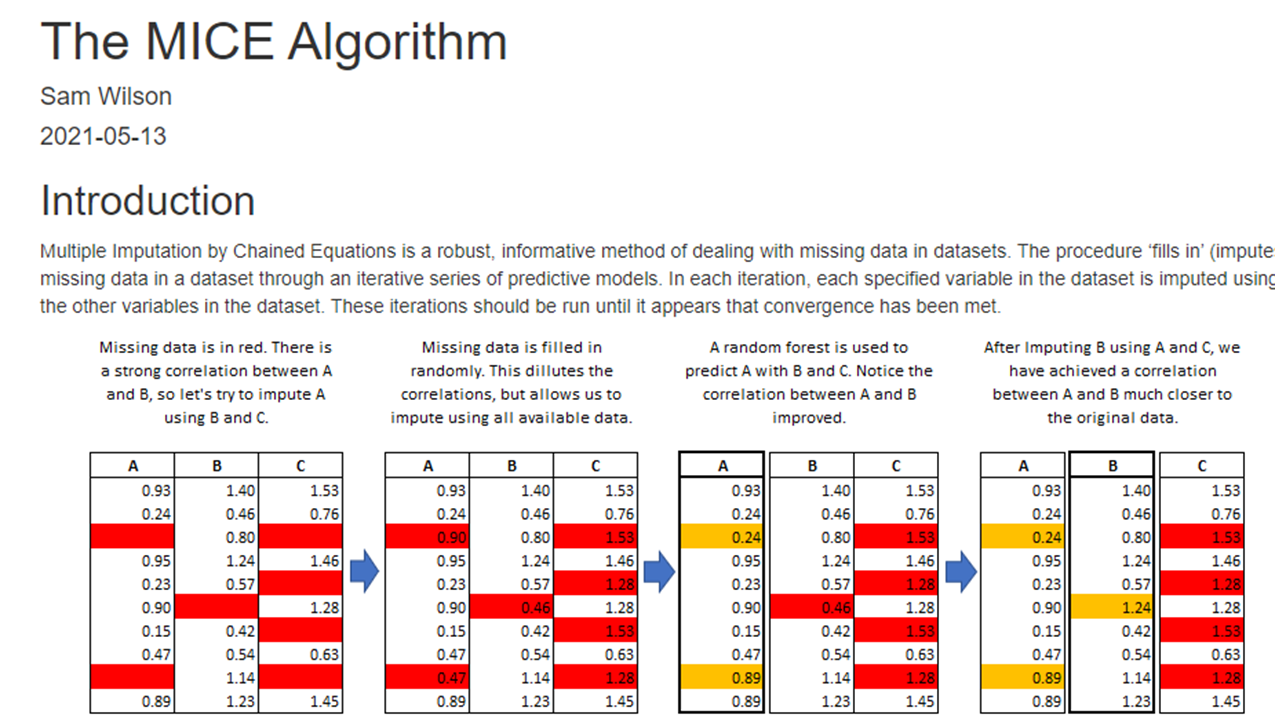
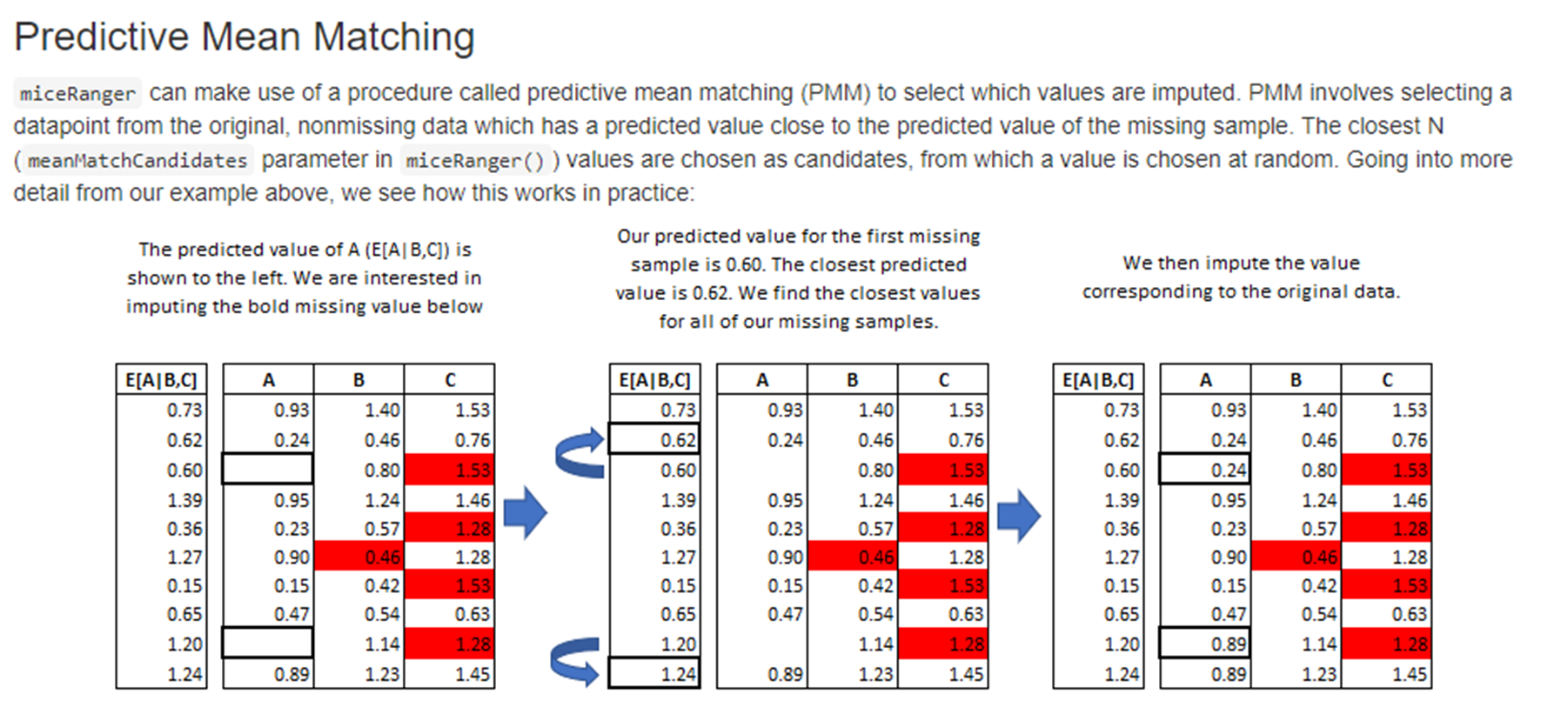Sourced from cran.r-project.org

Let us get some data where we can perform some imputations. But because we are working with Python, we will not use the above, but use sklearn’s imputer.

Code

## Let us look at the mtcars dataset

import statsmodels.api as sm
df = sm.datasets.get_rdataset('mtcars').data

Code

df

	mpg	cyl	disp	hp	drat	wt	qsec	vs	am	gear	carb
rownames
Mazda RX4	21.0	6	160.0	110	3.90	2.620	16.46	0	1	4	4
Mazda RX4 Wag	21.0	6	160.0	110	3.90	2.875	17.02	0	1	4	4
Datsun 710	22.8	4	108.0	93	3.85	2.320	18.61	1	1	4	1
Hornet 4 Drive	21.4	6	258.0	110	3.08	3.215	19.44	1	0	3	1
Hornet Sportabout	18.7	8	360.0	175	3.15	3.440	17.02	0	0	3	2
Valiant	18.1	6	225.0	105	2.76	3.460	20.22	1	0	3	1
Duster 360	14.3	8	360.0	245	3.21	3.570	15.84	0	0	3	4
Merc 240D	24.4	4	146.7	62	3.69	3.190	20.00	1	0	4	2
Merc 230	22.8	4	140.8	95	3.92	3.150	22.90	1	0	4	2
Merc 280	19.2	6	167.6	123	3.92	3.440	18.30	1	0	4	4
Merc 280C	17.8	6	167.6	123	3.92	3.440	18.90	1	0	4	4
Merc 450SE	16.4	8	275.8	180	3.07	4.070	17.40	0	0	3	3
Merc 450SL	17.3	8	275.8	180	3.07	3.730	17.60	0	0	3	3
Merc 450SLC	15.2	8	275.8	180	3.07	3.780	18.00	0	0	3	3
Cadillac Fleetwood	10.4	8	472.0	205	2.93	5.250	17.98	0	0	3	4
Lincoln Continental	10.4	8	460.0	215	3.00	5.424	17.82	0	0	3	4
Chrysler Imperial	14.7	8	440.0	230	3.23	5.345	17.42	0	0	3	4
Fiat 128	32.4	4	78.7	66	4.08	2.200	19.47	1	1	4	1
Honda Civic	30.4	4	75.7	52	4.93	1.615	18.52	1	1	4	2
Toyota Corolla	33.9	4	71.1	65	4.22	1.835	19.90	1	1	4	1
Toyota Corona	21.5	4	120.1	97	3.70	2.465	20.01	1	0	3	1
Dodge Challenger	15.5	8	318.0	150	2.76	3.520	16.87	0	0	3	2
AMC Javelin	15.2	8	304.0	150	3.15	3.435	17.30	0	0	3	2
Camaro Z28	13.3	8	350.0	245	3.73	3.840	15.41	0	0	3	4
Pontiac Firebird	19.2	8	400.0	175	3.08	3.845	17.05	0	0	3	2
Fiat X1-9	27.3	4	79.0	66	4.08	1.935	18.90	1	1	4	1
Porsche 914-2	26.0	4	120.3	91	4.43	2.140	16.70	0	1	5	2
Lotus Europa	30.4	4	95.1	113	3.77	1.513	16.90	1	1	5	2
Ford Pantera L	15.8	8	351.0	264	4.22	3.170	14.50	0	1	5	4
Ferrari Dino	19.7	6	145.0	175	3.62	2.770	15.50	0	1	5	6
Maserati Bora	15.0	8	301.0	335	3.54	3.570	14.60	0	1	5	8
Volvo 142E	21.4	4	121.0	109	4.11	2.780	18.60	1	1	4	2

Code

## Next, we replace a quarter of the values in the data with NaNs

for row in range(df.shape[0]):
    for col in range(df.shape[1]):
        if np.random.uniform() < 0.25:
            df.iloc[row,col] = np.nan

Code

df.describe()

	mpg	cyl	disp	hp	drat	wt	qsec	vs	am	gear	carb
count	22.000000	21.000000	22.000000	24.000000	26.000000	28.000000	26.000000	19.000000	22.000000	26.000000	26.000000
mean	20.104545	5.809524	219.818182	157.000000	3.607692	3.214357	18.044231	0.421053	0.454545	3.615385	3.038462
std	5.287765	1.778175	124.392748	70.173078	0.510453	1.011753	1.754980	0.507257	0.509647	0.697247	1.684773
min	10.400000	4.000000	75.700000	52.000000	2.760000	1.513000	14.600000	0.000000	0.000000	3.000000	1.000000
25%	15.950000	4.000000	120.475000	102.500000	3.150000	2.581250	17.020000	0.000000	0.000000	3.000000	2.000000
50%	19.200000	6.000000	163.800000	162.500000	3.695000	3.325000	17.990000	0.000000	0.000000	3.500000	3.000000
75%	22.800000	8.000000	313.750000	186.250000	3.920000	3.570000	18.900000	1.000000	1.000000	4.000000	4.000000
max	30.400000	8.000000	472.000000	335.000000	4.930000	5.424000	22.900000	1.000000	1.000000	5.000000	8.000000

9.28 Simple Imputer

Simple Imputer imputes values for a feature using only non-missing values in that feature dimension. Valid strategies are mean, median, most_frequent, constant.

Code

import numpy as np
from sklearn.impute import SimpleImputer
imp = SimpleImputer(missing_values=np.nan, strategy='mean')

Code

pd.DataFrame(imp.fit_transform(df), columns = df.columns, index = df.index).round(1)

	mpg	cyl	disp	hp	drat	wt	qsec	vs	am	gear	carb
rownames
Mazda RX4	21.0	6.0	160.0	157.0	3.9	2.6	16.5	0.0	1.0	4.0	4.0
Mazda RX4 Wag	21.0	6.0	160.0	157.0	3.9	2.9	17.0	0.4	1.0	3.6	4.0
Datsun 710	22.8	4.0	108.0	93.0	3.8	3.2	18.6	1.0	0.5	3.6	3.0
Hornet 4 Drive	20.1	6.0	258.0	157.0	3.6	3.2	19.4	1.0	0.5	3.6	1.0
Hornet Sportabout	18.7	5.8	360.0	175.0	3.2	3.4	17.0	0.0	0.0	3.0	2.0
Valiant	18.1	6.0	219.8	105.0	3.6	3.5	20.2	0.4	0.0	3.0	1.0
Duster 360	14.3	8.0	219.8	245.0	3.2	3.6	18.0	0.0	0.0	3.0	4.0
Merc 240D	24.4	4.0	219.8	62.0	3.7	3.2	20.0	1.0	0.0	4.0	3.0
Merc 230	22.8	4.0	140.8	95.0	3.9	3.2	22.9	0.4	0.5	4.0	2.0
Merc 280	19.2	6.0	167.6	123.0	3.9	3.4	18.3	1.0	0.0	4.0	4.0
Merc 280C	17.8	5.8	167.6	157.0	3.9	3.4	18.9	1.0	0.0	4.0	4.0
Merc 450SE	16.4	5.8	219.8	180.0	3.6	3.2	17.4	0.4	0.5	3.0	3.0
Merc 450SL	20.1	8.0	275.8	180.0	3.1	3.7	17.6	0.0	0.0	3.0	3.0
Merc 450SLC	20.1	5.8	219.8	180.0	3.1	3.2	18.0	0.0	0.5	3.6	3.0
Cadillac Fleetwood	20.1	8.0	472.0	205.0	2.9	5.2	18.0	0.0	0.0	3.0	4.0
Lincoln Continental	10.4	8.0	219.8	215.0	3.0	5.4	18.0	0.0	0.0	3.0	4.0
Chrysler Imperial	14.7	5.8	440.0	230.0	3.2	5.3	17.4	0.0	0.5	3.0	4.0
Fiat 128	20.1	4.0	219.8	157.0	4.1	2.2	19.5	0.4	1.0	4.0	1.0
Honda Civic	30.4	4.0	75.7	52.0	4.9	1.6	18.5	1.0	0.5	4.0	3.0
Toyota Corolla	20.1	5.8	219.8	157.0	3.6	1.8	18.0	1.0	0.5	4.0	3.0
Toyota Corona	20.1	4.0	120.1	157.0	3.7	2.5	20.0	1.0	0.0	3.0	1.0
Dodge Challenger	20.1	5.8	318.0	150.0	2.8	3.5	16.9	0.4	0.0	3.0	2.0
AMC Javelin	15.2	5.8	219.8	150.0	3.2	3.4	17.3	0.4	0.5	3.0	2.0
Camaro Z28	20.1	8.0	219.8	157.0	3.6	3.8	15.4	0.4	0.5	3.0	4.0
Pontiac Firebird	19.2	8.0	400.0	175.0	3.1	3.8	18.0	0.0	0.0	3.0	3.0
Fiat X1-9	27.3	4.0	79.0	66.0	4.1	1.9	18.9	0.4	1.0	4.0	1.0
Porsche 914-2	26.0	5.8	120.3	91.0	3.6	2.1	16.7	0.4	1.0	3.6	2.0
Lotus Europa	30.4	4.0	95.1	113.0	3.8	1.5	18.0	0.4	1.0	5.0	2.0
Ford Pantera L	15.8	5.8	351.0	264.0	4.2	3.2	18.0	0.0	1.0	5.0	4.0
Ferrari Dino	20.1	5.8	145.0	175.0	3.6	2.8	15.5	0.0	1.0	5.0	6.0
Maserati Bora	15.0	8.0	301.0	335.0	3.5	3.6	14.6	0.4	1.0	3.6	8.0
Volvo 142E	21.4	4.0	121.0	109.0	4.1	3.2	18.6	0.4	1.0	4.0	2.0

9.29 Iterative Imputer (sklearn)

The Iterative Imputer models each feature with missing values as a function of other features, and uses that estimate for imputation. It does so in an iterated round-robin fashion: at each step, a feature column is designated as output y and the other feature columns are treated as inputs X. A regressor is fit on (X, y) for known y.

Then, the regressor is used to predict the missing values of y.

This is done for each feature in an iterative fashion, and then is repeated for max_iter imputation rounds. The results of the final imputation round are returned.

Source: https://scikit-learn.org/stable/modules/impute.html#iterative-imputer

Code

# Note: IterativeImputer still requires the experimental import as of sklearn 1.x
# For most practical cases, KNNImputer (below) is a strong default and needs no experimental flag.
from sklearn.experimental import enable_iterative_imputer
from sklearn.impute import IterativeImputer
imp = IterativeImputer(max_iter=100, random_state=0)

Code

pd.DataFrame(imp.fit_transform(df), columns = df.columns, index = df.index).round(1)

	mpg	cyl	disp	hp	drat	wt	qsec	vs	am	gear	carb
rownames
Mazda RX4	21.0	6.0	160.0	110.0	3.9	3.3	16.5	0.4	1.0	4.0	4.0
Mazda RX4 Wag	21.0	6.0	116.4	110.0	3.9	2.9	17.8	0.5	0.7	4.2	4.0
Datsun 710	22.8	4.0	108.0	94.6	3.8	2.3	18.6	1.3	0.9	3.6	1.0
Hornet 4 Drive	21.4	6.0	258.0	170.1	3.1	3.2	19.4	0.7	0.0	3.0	1.0
Hornet Sportabout	18.7	7.5	360.0	175.0	3.2	4.4	18.2	0.0	0.0	3.0	2.0
Valiant	18.1	6.0	225.0	105.0	2.8	4.0	20.2	1.0	0.0	3.0	1.0
Duster 360	14.3	8.0	334.7	245.0	3.4	3.6	15.8	0.0	0.0	3.0	2.8
Merc 240D	24.1	5.3	146.7	62.0	3.7	3.2	19.8	1.0	0.0	4.0	2.0
Merc 230	22.8	4.0	140.8	95.0	3.9	3.2	22.9	1.0	0.8	4.0	2.0
Merc 280	19.2	6.0	167.6	123.0	3.9	3.4	18.3	1.0	0.0	4.0	4.0
Merc 280C	17.8	6.1	167.6	123.0	3.9	3.2	18.9	0.9	0.0	4.0	3.0
Merc 450SE	16.4	8.0	295.3	180.0	3.1	4.1	17.3	0.0	0.0	3.0	3.0
Merc 450SL	17.9	8.0	275.8	180.8	3.5	3.4	16.2	0.0	0.0	3.4	3.0
Merc 450SLC	17.9	8.0	275.8	180.0	3.1	3.8	18.0	0.0	0.0	3.0	3.0
Cadillac Fleetwood	10.4	8.1	472.0	280.3	3.1	5.6	18.0	0.0	0.0	3.0	4.0
Lincoln Continental	10.4	8.0	460.0	274.3	3.4	5.4	17.8	0.0	0.0	3.0	4.0
Chrysler Imperial	10.9	8.0	440.0	264.2	3.2	5.3	17.8	0.1	0.0	3.0	4.0
Fiat 128	32.4	4.0	78.7	66.0	4.1	1.6	19.5	1.0	0.7	4.0	1.0
Honda Civic	30.4	4.0	27.9	52.0	4.1	1.6	19.0	1.0	1.0	4.3	2.0
Toyota Corolla	27.9	4.0	41.1	65.0	3.9	1.8	19.9	1.0	1.0	4.0	1.7
Toyota Corona	24.6	4.0	120.1	97.0	3.7	2.5	20.0	1.0	1.1	3.0	0.7
Dodge Challenger	16.1	8.0	318.0	201.8	2.8	3.8	16.9	0.0	0.0	2.8	2.0
AMC Javelin	15.2	8.0	304.0	150.0	3.2	4.2	17.3	0.0	0.0	3.0	2.0
Camaro Z28	13.3	8.0	350.0	218.5	3.7	3.8	16.2	0.0	0.0	3.0	2.4
Pontiac Firebird	19.2	7.6	286.4	175.0	3.1	3.5	17.0	0.0	0.2	3.0	2.0
Fiat X1-9	27.3	4.0	79.0	66.0	4.1	1.9	18.9	1.0	1.0	3.8	1.0
Porsche 914-2	26.0	5.9	120.3	91.0	4.4	1.9	16.4	0.0	1.0	3.8	2.0
Lotus Europa	30.4	4.0	95.1	113.0	4.5	1.5	16.9	1.0	1.0	5.0	2.8
Ford Pantera L	14.7	8.0	351.0	219.0	4.2	3.2	14.5	0.0	-0.2	2.8	1.6
Ferrari Dino	23.4	6.0	124.9	175.0	3.6	2.8	17.1	0.4	1.0	4.9	6.0
Maserati Bora	14.9	8.0	301.0	335.0	3.5	3.6	14.6	-0.3	1.0	5.0	8.0
Volvo 142E	24.4	5.2	121.0	109.0	4.1	2.8	18.6	0.5	1.0	4.0	3.7

Let us compare imputed results to actual results in our original data.

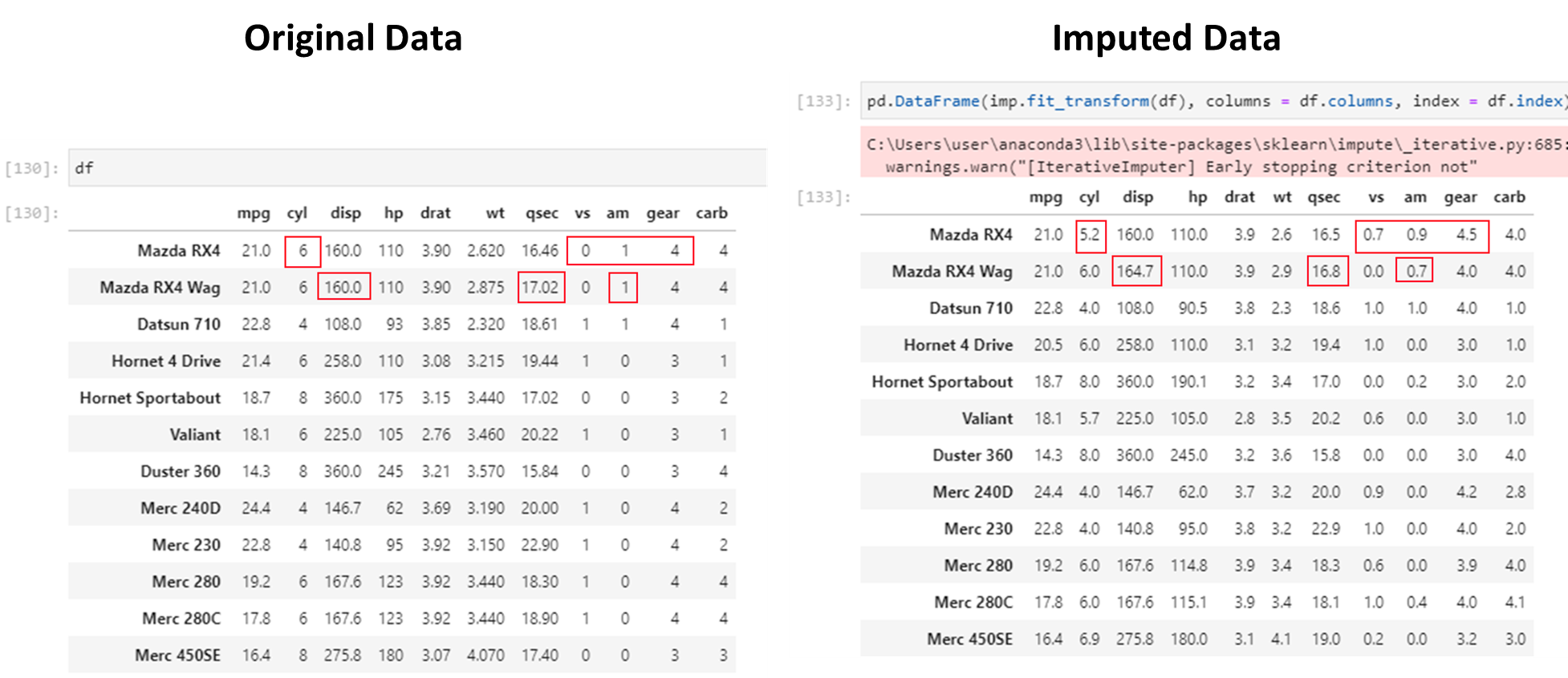
Not bad!!

9.30 KNN Imputer

The KNNImputer class provides imputation for filling in missing values using the k-Nearest Neighbors approach. By default, a euclidean distance metric that supports missing values, nan_euclidean_distances, is used to find the nearest neighbors.
Each missing feature is imputed using values from n_neighbors nearest neighbors that have a value for the feature.
The feature of the neighbors are averaged uniformly or weighted by distance to each neighbor.
- When the number of available neighbors is less than n_neighbors and there are no defined distances to the training set, the training set average for that feature is used during imputation.
- If there is at least one neighbor with a defined distance, the weighted or unweighted average of the remaining neighbors will be used during imputation.
- If a feature is always missing in training, it is removed during transform.

Source: https://scikit-learn.org/stable/modules/impute.html#knnimpute

9.30.1 Data Validation Frameworks

Beyond handling missing values, robust analytics pipelines include data validation. Key tools:

ydata-profiling (pip install ydata-profiling): Auto-generates a full HTML report on any DataFrame — distributions, missing values, correlations, outliers.
```
from ydata_profiling import ProfileReport
report = ProfileReport(df, title="Data Quality Report")
report.to_file("report.html")
```
Great Expectations (pip install great-expectations): Define and enforce data quality rules programmatically. Ideal for production pipelines where bad data must be caught early.
Pandera (pip install pandera): Lightweight schema validation for pandas DataFrames. Catches type errors and constraint violations before they reach your model.

Code

from sklearn.impute import KNNImputer
imputer = KNNImputer(n_neighbors=2, weights="uniform")
pd.DataFrame(imputer.fit_transform(df), columns = df.columns, index = df.index)

	mpg	cyl	disp	hp	drat	wt	qsec	vs	am	gear	carb
rownames
Mazda RX4	21.00	7.0	160.00	145.0	3.900	3.3025	16.46	0.0	1.0	4.0	3.5
Mazda RX4 Wag	21.00	6.0	160.00	110.0	3.900	2.8750	17.95	0.5	1.0	4.0	4.0
Datsun 710	22.80	5.0	108.00	93.0	3.850	3.3925	17.64	1.0	0.0	4.0	1.0
Hornet 4 Drive	20.45	6.0	292.50	118.5	3.535	3.2150	19.44	1.0	0.0	3.0	2.5
Hornet Sportabout	15.80	7.0	360.00	175.0	3.150	3.4400	17.64	0.5	0.0	3.0	3.5
Valiant	18.10	6.0	225.00	121.0	3.140	3.4600	19.72	1.0	0.0	3.0	1.0
Duster 360	14.30	7.0	317.90	177.5	3.210	3.5700	15.84	0.5	0.0	3.0	4.0
Merc 240D	19.80	5.0	172.55	62.0	4.315	2.8400	20.00	1.0	0.0	4.0	1.0
Merc 230	24.85	4.0	140.80	64.0	3.920	2.7075	22.90	1.0	0.0	4.0	2.0
Merc 280	24.85	6.0	167.60	92.5	3.920	3.4400	18.30	1.0	0.0	4.0	3.5
Merc 280C	17.65	6.0	167.60	123.0	3.920	3.3275	18.87	1.0	0.0	4.0	4.0
Merc 450SE	15.80	8.0	275.80	180.0	3.070	4.0700	17.80	0.0	0.0	3.0	3.0
Merc 450SL	17.30	8.0	275.80	180.0	3.070	3.7300	17.60	0.0	0.0	3.0	3.0
Merc 450SLC	15.80	8.0	275.80	180.0	3.070	3.9000	18.00	0.0	0.0	3.0	3.0
Cadillac Fleetwood	10.40	7.0	472.00	205.0	2.930	5.2500	17.98	0.0	0.0	3.0	4.0
Lincoln Continental	10.40	8.0	460.00	215.0	3.000	5.4240	17.82	0.0	0.0	3.0	4.0
Chrysler Imperial	14.70	7.0	440.00	230.0	3.230	5.3450	17.42	0.5	0.0	3.0	4.0
Fiat 128	32.40	4.0	105.95	66.0	4.080	2.2000	21.40	1.0	0.5	4.0	1.0
Honda Civic	30.40	4.0	75.70	64.0	4.930	1.6150	18.52	1.0	1.0	4.0	2.0
Toyota Corolla	31.40	4.0	71.10	65.0	4.220	1.8350	19.90	1.0	1.0	4.0	1.0
Toyota Corona	21.50	4.0	120.10	121.0	3.700	2.4650	20.01	1.0	0.5	3.0	1.0
Dodge Challenger	15.50	7.0	318.00	150.0	2.760	3.5200	16.87	0.5	0.0	3.0	2.0
AMC Javelin	15.20	8.0	304.00	150.0	3.150	3.4350	17.30	0.0	0.0	3.0	2.0
Camaro Z28	13.30	8.0	350.00	245.0	3.730	3.8400	15.41	0.5	0.0	3.0	4.0
Pontiac Firebird	19.20	8.0	400.00	175.0	3.140	3.8450	17.05	0.0	0.0	3.0	2.0
Fiat X1-9	27.30	4.0	79.00	64.0	4.080	1.9350	18.90	1.0	1.0	3.5	1.0
Porsche 914-2	26.00	4.0	120.30	64.0	4.430	2.1400	19.30	0.0	0.5	5.0	1.5
Lotus Europa	30.40	5.0	95.10	113.0	3.770	1.5130	19.17	1.0	1.0	3.0	2.0
Ford Pantera L	15.80	8.0	351.00	212.5	4.220	3.1700	14.50	0.0	0.0	3.0	4.0
Ferrari Dino	19.70	6.0	145.00	175.0	3.140	3.4725	15.50	0.5	1.0	5.0	6.0
Maserati Bora	15.05	8.0	301.00	335.0	3.540	3.3925	14.60	0.0	0.0	5.0	8.0
Volvo 142E	29.20	4.0	121.00	64.0	4.255	2.7800	18.60	1.0	1.0	4.0	2.0

Let us compare imputed values to actual data.

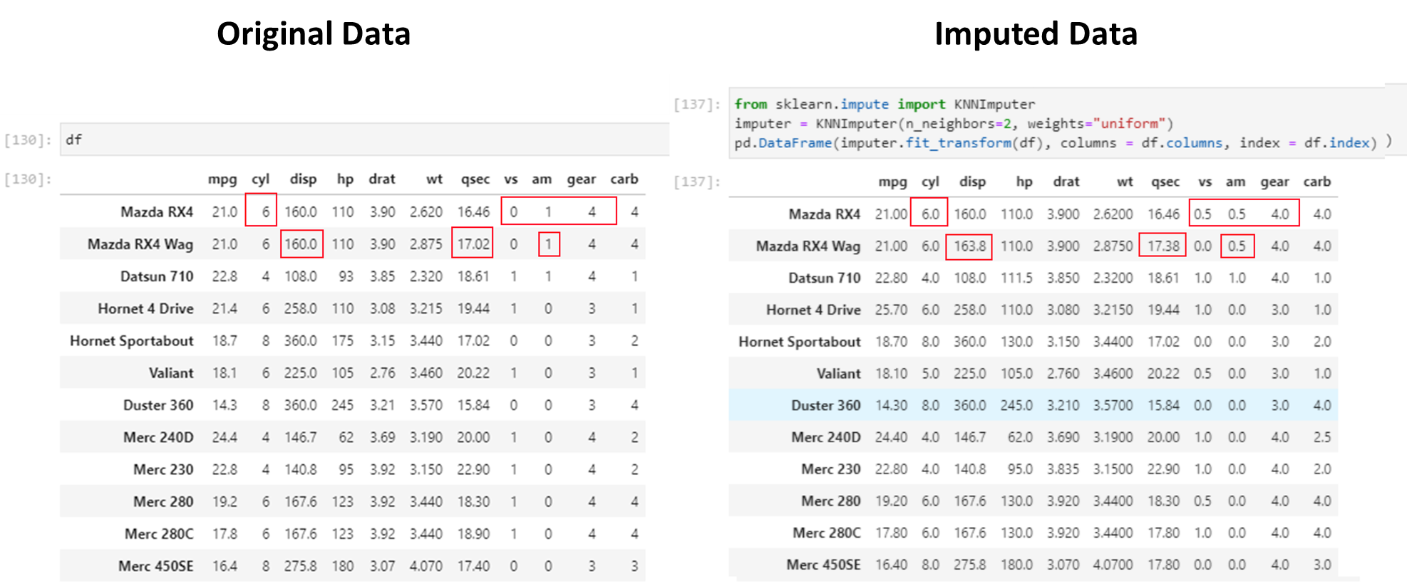
This is even better than the iterative imputer!!

9.31 List Comprehension and Other Useful Tricks

List comprehension returns a list, and takes the following format:

[** function(item) for item in iterable if condition **]

Code

# Create an empty dataframe

import pandas as pd

df = pd.DataFrame(columns = ['Date', 'User 1', 'User 2', 'User 3', 'User 4', 'User 5', 'User 6', 'User 7'])
df

	Date	User 1	User 2	User 3	User 4	User 5	User 6	User 7

Code

# List all columns in a dataframe meeting a criteria

[col for col in df if col.startswith('U')]

['User 1', 'User 2', 'User 3', 'User 4', 'User 5', 'User 6', 'User 7']

Code

# If condition in a single line

b = 4
a = "positive" if b >= 0 else "negative"
a

'positive'

List comprehension
newlist = [expression for item in iterable if condition == True]

Code

# Basic list comprehension
x = list(v**2 for v in range(4))
x

[0, 1, 4, 9]

Code

# List comprehension

fruits = ["apple", "banana", "cherry", "kiwi", "mango"]

newlist = [x for x in fruits if "a" in x]

print(newlist)

['apple', 'banana', 'mango']

# Subsetting a dict

samples = {k: v for k, v in samples.items() if k not in ["idx", "sentence1", "sentence2"]}

Code

# A function to identify text in a string
def corona(text):
    corona_story_strings = ['covid', 'corona', 'sars', 'virus', 'coronavirus', 'vaccine']
    return any(x in text for x in corona_story_strings)

9.1 Data Manipulation, Transformation and Cleaning

9.2 Reshaping Data

9.2.1 Modern Data Tooling

9.3 The Setup

9.3.1 Create a DataFrame

9.3.2 Read the diamonds and mtcars dataframes

9.4 Selecting columns

9.5 Select rows (queries)

9.6 Subsetting with loc and iloc

9.7 Understanding Data Types

9.8 Change column to categorical

9.8.1 How to list categories

9.9 Get column names

9.10 Add Columns

9.10.1 Add column with insert

9.10.2 Add column with assign

9.11 Delete Columns

9.12 Reordering Columns

9.13 Sorting Values

9.14 Renaming Columns

9.15 Removing Duplicates

9.16 Replacing Values

9.17 Binning using Pandas cut Function

9.18 Binning into Quantiles using qcut

9.19 Select a random sample of data

9.20 String operations with Pandas

9.21 Value Counts

9.22 Extract unique values

9.22.1 Fuzzy String Matching

9.23 Groupby

9.23.1 rename columns with Groupby

9.23.2 Named Aggregations (Preferred Style)

9.24 Joining Data with Merge

9.24.1 Left Join

9.24.2 Right Join

9.24.3 Inner Join

9.24.4 Outer Join

9.24.5 Cross Join

9.25 Concatenation

9.25.1 Concatenation example

9.26 Dealing with Missing Values

9.26.1 Understanding the extent of missing values

9.26.2 How to think about missing values

9.26.2.1 Drop Missing Values

9.26.2.1.1 Drop rows with missing values

9.26.2.1.2 Drop columns with missing values

9.26.2.2 Fill Missing Data

9.26.3 Forward and Backward Fill

9.27 Imputation using sklearn

9.28 Simple Imputer

9.29 Iterative Imputer (sklearn)

9.30 KNN Imputer

9.30.1 Data Validation Frameworks

9.31 List Comprehension and Other Useful Tricks

9.6 Subsetting with `loc` and `iloc`

9.10.1 Add column with `insert`

9.10.2 Add column with `assign`

9.17 Binning using Pandas `cut` Function

9.18 Binning into Quantiles using `qcut`

9.23.1 `rename` columns with Groupby